---
title: 'A Guide to Reliability: Avoiding Misconceptions'
author: "Derek C. Briggs and Claude Code (Opus 4.6 & 4.7)"
output:
html_document:
code_folding: hide
toc: yes
toc_float:
collapsed: yes
smooth_scroll: yes
pdf_document:
toc: yes
word_document:
toc: yes
fontsize: 11pt
---
```{r inject-rootdir, include=FALSE}
knitr::opts_knit$set(root.dir = "/Users/briggsd/Library/CloudStorage/Dropbox/Github/Measurement and Psychometrics/Reliability/R Markdown Tutorial")
```
```{r global_options, include=FALSE}
knitr::opts_chunk$set(warning=FALSE, message=FALSE,
tidy.opts=list(width.cutoff=50))
```
*****
# Motivation for this Document
For many years now I've taught the concept of reliability to graduate students as part of an educational measurement sequence here at the University of Colorado. Beyond formal readings, the materials I've given students to help them study have typically consisted of powerpoint slides. While I think the content on those slides has gotten better and better over time, I think the R Markdown format is a far superior format because of the way it allows one to integrate narrative and empirical demonstrations in a single place. The other push came from a special focus article and commentaries on reliability I helped put together when I was still the editor of *Educational Measurement: Issues and Practice* in 2015.
My hope is that the "learning module" that follows will build on these articles and thereby serve as a useful resource in developing a deep understanding of both the concept of reliability, and ways that this concept can be parameterized and estimated.
# Introduction
Reliability is one of the most important concepts in measurement. Let's start with the intuition behind reliability for measurements taken in the physical sciences. The concept of reliability is premised on replication. It goes something like this: say I devise a measurement procedure. By procedure, I mean a set of steps that need to be taken in order produce a measure of some attribute of interest for a given object of interest. The procedure culminates in a numeric value. When we ask about the reliability of the value, we are essentially asking how likely we would be to observe the same value if the measurement procedure were to be replicated. But this raises some thorny questions. If we replicate the procedure, what stays fixed and what varies? Time, for instance, cannot be fixed, but can we treat the passage of time as irrelevant to the procedure? What about the instrument used to take the measure, is that fixed? What about the person operating the instrument? What about other conditions, such as the location where the measurement procedure is taking place? The object being measured?
You can see already that what it is we mean when we speak of "reliability" depends greatly on being clear about the conditions of measurement and, conceptually, what is and is not being replicated. This is certainly true in the context of physical measurement, and equally true in educational and psychological measurement.
The concept of reliability in psychometrics has it origins in what is known as *True Score Theory* (also referred to as *Classical Test Theory*). True score theory is really a means to an end: it provides a mathematical basis to operationalize the concept of reliability into a model parameter. This parameter is a reliability coefficient, something that can be estimated from data. In what follows I will try to take you through this derivation, but I'm going to take the liberty of borrowing from the conceptual toolbox of *Generalizability Theory* (Cronbach et al, 1972) so if you pay close attention you'll see that this derivation is not exactly the same as the classic formulation found in Lord & Novick.
# True Score Theory
## Preliminaries
Let's start with a "test" score, $X$, associated with a test-taker, indexed by the subscript $j$. A test in this context consists of some fixed number of items, and the responses to these items are given ordinal scores. (In this sense we can also consider an attitudinal survey to be a type of test). So if we then let the subscript $i$ index a test item, then
$$ X_j= \sum_{i=1}^{n_i} X_{ij} $$
where $n_i$ represents the total number of items on the test.
In much of what you are going to see in the derivation of the classical test theory model, test items are going to disappear from view: the theory occurs at the level of a test score, where a test score is computed as either a sum or average across items. But in order to make sense of the concept of "measurement error", it's really important to be able to think of the existence of a hypothetical "universe" of items that *could* have been placed on the test. (This is an instance when I'm borrowing from Generalizability Theory.) In this sense, the $n_i$ that happen to be on a given test are just a random sample from a universe of $I$ items. We could just as easily have created a test comprised of $n^\prime_i$ items, and if we did, we'd expect the two tests to be *parallel* in the sense that they should be equally difficult, on average, and that the test scores should have the same variance, on average. So there are two sources of chance variability that influence the value we observe for $X_{ij}$: the sampling of test-takers from some population of test-takers, and the sampling of items from some universe of items.
## The Within-Person Model
For each test-taker, let's assume that an observed test score is a linear function of a "true score" and "error"
$$\tag{1}X_j = \tau_j + e_j$$
Each person's true score, $\tau_j$, is *defined* as the expected value taken over all possible tests of $n_i$ items that could be constructed by sampling at random (with replacement) from the universe of possible test items.
$$\tag{2}E(X_j)=\tau_j$$
Therefore the "error" term simply represents the difference between a person's observed score and the (unknown) true score
$$\tag{3}e_j=X_j-E(X_j)$$
Note that $\tau_j$ and $e_j$ are independent across replications of the testing procedure with new samples of items, and therefore uncorrelated, by definition. This is because $\tau_j$ is a constant and $E(e_j)=0$. This represents an untestable assumption, something that cannot be falsified with data.
Now, what we'd really like to know about, for each test-taker ($j$), is the sampling distribution of test scores we would observe if it were possible to have the person take tests with different sets of items over and over again, but after each administration we "brainwash" the person to forget the experience.
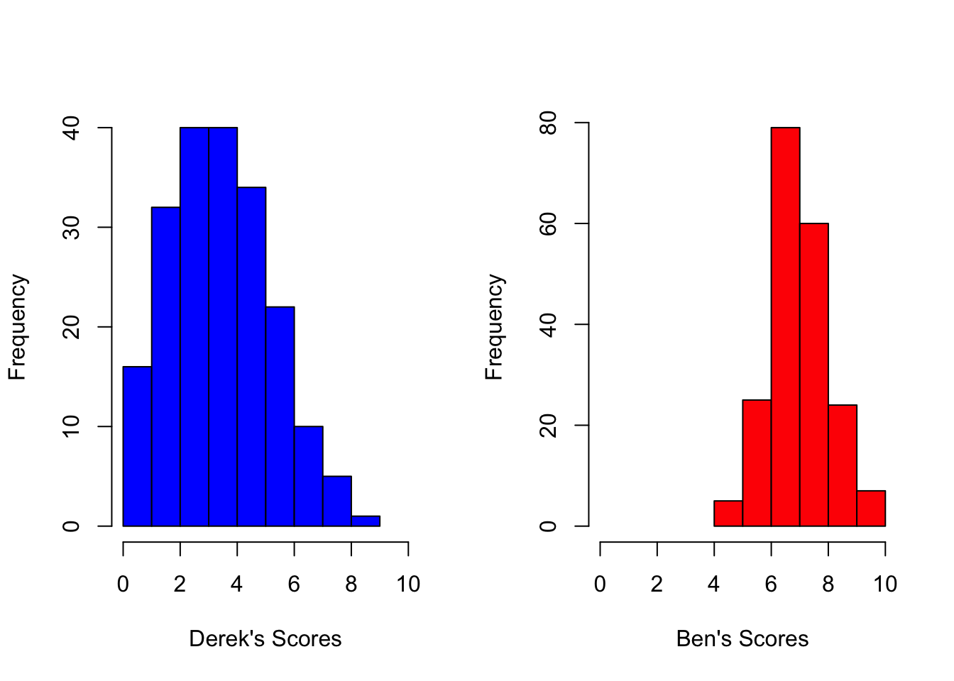
Let's consider the hypothetical example of two students, Derek and Ben. Both take a vocabulary test consisting of 10 items. How would their scores (number of items correct out of 10) vary if they took 200 vocabulary tests, each time with a different random sample of items? (I'm just picking 200 tests out of the air here because I need a finite value to simulate data; I could just as well have picked 1000 or 10000000--this has no impact on the point I'm about to make.)
```{r}
library(msm)
set.seed(8971)
derek<-rtnorm(200,3.3,2,lower=0,upper=10)
derek<-round(derek,digits=1)
set.seed(1234)
ben<-rtnorm(200,7.1,1,lower=0,upper=10)
ben<-round(ben,digits=1)
par(mfrow=c(1,2))
hist(derek,xlim=range(0,10),main='',col="blue",xlab="Derek's Scores")
hist(ben,xlim=range(0,10),breaks=c(4:10),main='',col="red",xlab="Ben's Scores")
```
Two things to notice here.
1. Derek's true score (3.3) is lower than Ben's true score (7.1)
2. The variability in Derek's scores (SD=2) is twice as big as that for Ben's scores (SD=1)
We can formalize this result by turning back to the fundamental equation of true score theory, $X_j = \tau_j + e_j$. If we are interested in the sampling variance of observed scores for each case $j$, we want
$$\sigma^2_{X_j}=\sigma^2_{\tau_j}+\sigma^2_{e_j}$$
since $\tau_j$ and $e_j$ are independent. But since $\tau_j$ is a constant, this expression reduces to
$$\sigma^2_{X_j}=\sigma^2_{e_j}$$
In words, for each case, variance in observed scores across replications of the measurement procedure is caused solely by error variance.
Let Derek represent case 1 $(j=1)$, and Ben represent case 2 $(j=2)$. In our hypothetical example, $\sigma_{e_1}>\sigma_{e_2}$, which means that not only is Derek's true score lower than Ben's true score, it is measured with more error than Ben's.
## Conceptual Issues
This raises two questions.
1. What is the cause of measurement error in this scenario?
One typical answer to this is to point to idiosyncratic unpredictable features of the testing experience that can affect test-takers differently (e.g., getting a good or bad night of sleep, happening to sit next to someone with a distracting cough). This is possible (and it certainly reflects what the early developers of CTT had in mind), but it doesn't seem entirely consistent with the thought experiment that would give rise to a distribution of scores for each test-taker. The only thing that is clearly changing in each replication of the measurement procedure is the set of items to which a test-taker is being exposed. Everything else about the testing experience stays constant--the day, the time of day, the surrounding environment, etc. These things still might have an impact on a student's performance, but they would become part of the student's true score (biasing it up or down). However, perhaps it is possible to imagine that whenever a student is asked to recall a word, or perform any kind of cognitive task for that matter, that there is some randomness involved, something unpredictable, and this can cause a student to get a task right on some occasions but not others.
The clearest source of "error variance" in this context comes in the interaction between a test-taker and the particular set of items included on the test. Think of it this way: if any 10 item test is a random sample from a universe of possible items we could have used on the test, then just by chance, on any given test some people will see items that happen to be easier for them, and some will see items that happen to be harder for them. (Example: On one test a student gets a vocabulary item that happens to be something that was in a book she read for fun over the summer, on another test she doesn't.) So what we mean by measurement error is probably best understood as the positive or negative bump in an observed score that can be attributed to a person's good or bad luck in the items that happen to be on the test when it is administered.
2. Why would measurement error be bigger or smaller for certain test-takers?
Well, what if measurement error is not independent of test-takers' true score as it has been defined in this model--maybe it's bigger for students with low true scores, and smaller for students with high true scores. This is a nice transition to the heart of classical test theory as a statistical problem: *we have no good way to get person-specific estimates of measurement error*. The problem is that we can't actually observe within-person distributions of observed scores because (a) we can't administer an infinite (or even a very large) number of tests with different random sets of items, and (b) even if we could, the test scores wouldn't be independent. Test-takers might tire, or they might learn as they go.
So the strategy we take in true score theory is to formulate a model at the population level, use this to compute a reliability coefficient, and then use this reliability coefficient to back out an estimate of average measurement error for a given measurement procedure.
## The Between-Person Model
We are going to express the fundamental equation of true score theory for a population of test-takers as
$$\tag{4}X = T + E$$
This time, we are taking the variance not over replications within each individual test-taker, but *across* the observed scores of all individual test-takers.
$$\tag{5}\sigma^2_{X}=\sigma^2_{T}+\sigma^2_{E}$$
Recall that when the model was within-person, each person's true score was a constant ($\tau_j$). But here, since we are taking variance *across* people, it is not. Also, $\sigma^2_{E}$ can be thought of as $E[\sigma^2_{e_j}]$
## Conceptualizing the Sample as a Box Model
In moving to this population level model, we have to assume that each person for whom we have a score is a random sample from this population.

## Back to the Vocabulary Test Example
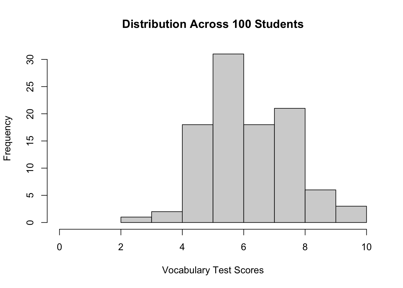
To be as concrete as I can here, let's go back to our hypothetical vocabulary test that Derek and Ben have taken. Derek and Ben were part of a sample of 100 students that took this test. The average score on this test was 6.4 with a standard deviation of 1.5.
```{r}
library(msm)
set.seed(345)
x<-rtnorm(100,6.4,1.5,lower=0,upper=10)
x<-round(x,digits=1)
hist(x,xlim=range(0,10),main="Distribution Across 100 Students",
     xlab="Vocabulary Test Scores")
```
The variability we observe in these scores is caused by *both* true differences among students, and by measurement error. So this brings us--finally--to the concept of reliability.
## The Concept of a Reliability Coefficient
$$\tag{6}\rho^2_{XT}=\frac{\sigma^2_{T}}{\sigma^2_{X}}$$
In words, reliability is the proportion of observed score variance that is true score variance. Another, more mathematical interpretation, is that reliability is the squared correlation we would get if it were possible to regress observed scores on true scores. Here are three mathematically equivalent formulations of the concept
$$\rho^2_{XT}=\frac{\sigma^2_{XT}}{\sigma^2_{X}\sigma^2_{T}}=\frac{\sigma^2_{T}}{\sigma^2_{T}+\sigma^2_{E}}=1-\frac{\sigma^2_{E}}{\sigma^2_{X}}$$
## Parallel Test Forms
It is crucial to appreciate that so far what we have done is establish a model that relates observed test scores to true scores and error, and then used this relationship to formulate what it means to have a test that produces reliable scores. What we have at this point is to identify the parameter of interest, $\rho^2_{XT}$. What we need is a way to get a good estimate of this parameter, since we can't directly observe either $\sigma^2_{T}$ or $\sigma^2_{E}$.
To do this, we need to introduce something that was alluded to above, and that is the notion of *parallel test forms*.
Let $X$ and $X^\prime$ represent two different test forms. The two test forms are parallel so long as $E(X)=E(X^\prime)=T$ and $\sigma^2_{X} = \sigma^2_{X^\prime}$. This means that the two forms are equivalent in difficulty and have the same observed score variance.
What if we compute the correlation of scores across the common population taking the two test forms? This correlation would be
$$\rho_{XX^\prime}=\frac{\sigma_{XX^\prime}}{\sigma_{X}\sigma_{X^\prime}}$$
Recall that $X = T + E$ and $X^\prime = T + E^\prime$, so we can rewrite the expression above as
$$\rho_{XX^\prime}=\frac{\sigma_{(T+E)(T+E^\prime)}}{\sigma_{X}\sigma_{X^\prime}},$$
$$\rho_{XX^\prime}=\frac{\sigma_{TT}+\sigma_{TE}+\sigma_{TE^\prime}+\sigma_{EE^\prime}}{\sigma_{X}\sigma_{X^\prime}}.$$
By assumption of the model, true scores and error scores are uncorrelated, and error scores are uncorrelated across parallel forms. So this expression reduces to
$$\rho_{XX^\prime}=\frac{\sigma_{TT}}{\sigma_{X}\sigma_{X^\prime}}.$$
Now the covariance between true scores is just the variance of true scores, so $\sigma_{TT}=\sigma^2_{T}$. And we defined parallel forms to have equal observed score variance, so $\sigma_{X}=\sigma_{X^\prime}$ and $\sigma_{X}\sigma_{X^\prime}=\sigma^2_{X}$. This means that
$$\tag{7}\rho_{XX^\prime}=\frac{\sigma^2_{T}}{\sigma^2_{X}}.$$
Which is pretty nice, because it means that $\rho_{XX^\prime}=\rho^2_{XT}$. So if we could create parallel test forms and correlate them, this would be equivalent to computing the squared correlation between true scores and observed scores, which is also equivalent to finding the proportion of observed score variance that is true score variance.
## Technical Aside on Derivation of the Spearman-Brown "Prophecy" Formula (this can be skipped)
If we have two random variables, ${Y_1}$ and ${Y_2}$ and then add them together to get a new variable $Y_3$, then $var(Y_3)=\sigma^2_{Y_1}+\sigma^2_{Y_2}+2\sigma_{Y_1 Y_2}$
Remember that correlation is just a standardized version of covariance, where
$$\rho_{Y_1 Y_2}=\frac{\sigma(Y_1,Y_2)}{\sigma_{Y_1}\sigma_{Y_2}}$$
In what follows it will be convenient to re-arrange terms such that
$$\sigma(Y_1,Y_2) = \rho_{Y_1 Y_2}\sigma_{Y_1}\sigma_{Y_2}$$
In words, the covariance of two random variables equals the correlation multiplied by product of each variable's standard deviation. OK, now let's get into the weeds.
Say we form a new composite test by adding together two tests of the same length. Let's define $X = Y_1 + Y_2$, $T = T_1 + T_2$ and $E = E_1 + E_2$
The variance of the composite observed score $X$ will be
$$\sigma^2_{X}=\sigma^2_{Y_1}+\sigma^2_{Y_2}+2\rho_{Y_1 Y_2}\sigma_{Y_1}\sigma_{Y_2}$$
the variance of the composite true score $T$ will be
$$\sigma^2_{T}=\sigma^2_{T_1}+\sigma^2_{T_2}+2\rho_{T_1 T_2}\sigma_{T_1}\sigma_{T_2}$$
and the variance of the composite error score $E$ will be
$$\sigma^2_{E}=\sigma^2_{E_1}+\sigma^2_{E_2}$$
Notice that the composite error term variance does not contain the covariance between the two subcomponents because we assume the error of two different tests are uncorrelated.
Now if $Y_1$ and $Y_2$ are parallel tests the three expressions above simplify as follows
$$\sigma^2_{X}=2\sigma^2_{Y_1}[1+\rho_{Y_1 Y^\prime_1}]$$
$$\sigma^2_{T}=4\sigma^2_{T_1}$$
$$\sigma^2_{E}=2\sigma^2_{E_1}$$
Key Insight: If we double the test length, true score variance increases twice as much as error variance.
## The Spearman-Brown Formula
The Spearman-Brown "prophecy" formula can be use to predict the reliability of a test that consists of a composite from two smaller tests of the same length (i.e., same number of items).
$$\tag{8}\rho_{XX^\prime}=\frac{2\rho_{YY^\prime}}{1+\rho_{YY^\prime}}$$
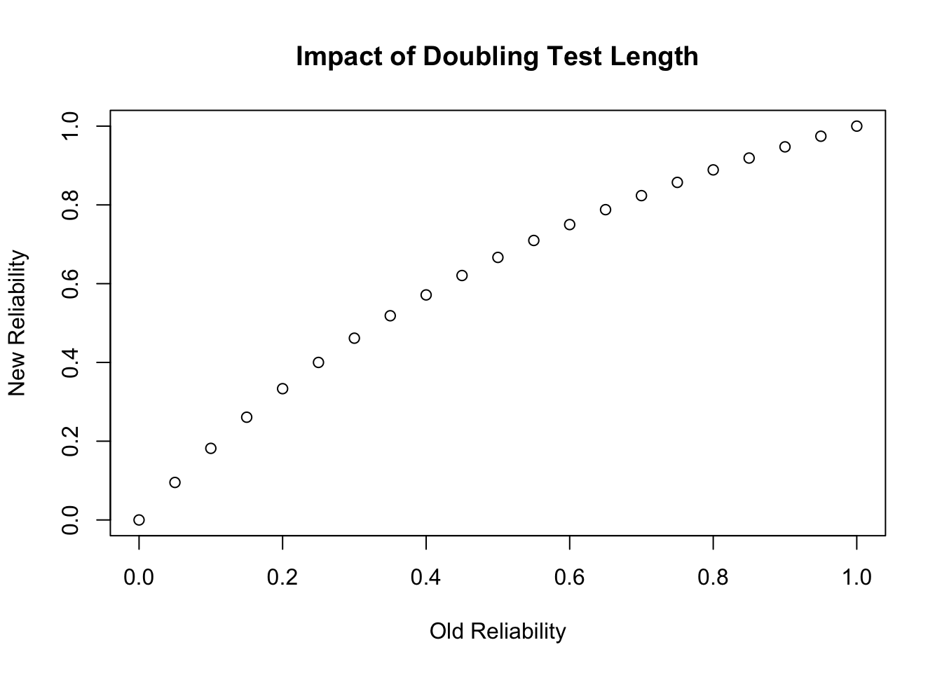
In the expression above, the composite test score $X=Y_1+Y_2$, and we define $Y_1$ and $Y_2$ to be parallel. So $X=Y+Y^\prime$. Think of $\rho_{YY^\prime}$ as the "old" reliability of a test and $\rho_{XX^\prime}$ as the "new" reliability we would predict if the test doubled in length.
```{r}
rel.old<-seq(from=0, to=1,by=.05)
rel.new<-2*rel.old/(1+rel.old)
plot(rel.old,rel.new,xlab="Old Reliability",ylab="New Reliability",
     main="Impact of Doubling Test Length")
```
Notice the nonlinear relationship. As base reliability increases, doubling the number of items is predicted to have less of an impact on the reliability of the new test.
So here is, historically speaking, the first practical strategy that was implemented for getting an estimate of reliability if you only have a single test administration.
1. Split the test into two parallel halves
2. Correlate the scores on each half
3. Use the Spearman-Brown formula to get an estimate for reliability if the test was twice as long.
Here is the formula for the *generalized Spearman-Brown prophecy*:
$$\tag{9}\rho_{XX^\prime}=\frac{k\rho_{YY^\prime}}{1+(k-1)\rho_{YY^\prime}}$$
This formula indicates how reliability is predicted to increase for any factor $k$ increase in the number of items on the test. We'll come back to the relationship between number of items and reliability again in the next section.
# Cronbach's Alpha
A problem with estimating reliability by splitting one test into two parallel forms is that it may not be obvious which split to use. Cronbach's alpha solves this problem by providing an estimate which can be interpreted as the average of all possible ways the test could be split into two forms and correlated, corrected for the restriction in test length. Here's the formula:
$$ \tag{10}\alpha = \frac{m}{m-1} \left(1-\frac{\sum_{i=1}^{m}S^2_{X_i}}{S^2_{X}} \right) $$
It is often typical to see this same formula with $\sigma^2_{X_i}$ in place of $S^2_{X_i}$ and $\sigma^2_{X}$ in place of $S^2_{X}$. Here I'm using the notation found in Davenport et al (2015) where they use $S$ in place of $\sigma^2$, probably to make the point that $\alpha$ is always an estimate based on computations after taking a sample of individual test-takers from some target population.
OK, let's unpack the equation for $\alpha$ by focusing first on the ratio inside the parenthesis.
1. The denominator, $S^2_{X}$ represents the variance of the composite test score we get by adding together all the items on the test. Since each item can be thought of as a random variable (recall the notion that each test is a random sample from a universe of possible items), it follows that $S^2_{X}=\sum_{i=1}^{m}\sum_{j=1}^{m}S_{X_iX_j}$. What this means is that the variance of the composite is the sum of all the item variances and item covariances. If there are $m$ items, then variance of the sum of these items equals the sum of $m^2$ variance and covariance terms.
2. The numerator, $\sum_{i=1}^{m}S^2_{X_i}$, represents the sum of all $m$ item variances. What it does _not_ include are the item covariances.
* When the ratio $\frac{\sum_{i=1}^{m}S^2_{X_i}}{S^2_{X}}$ is small, this implies that the covariance between test items is large.
* When the ratio $\frac{\sum_{i=1}^{m}S^2_{X_i}}{S^2_{X}}$ is large, this implies that the covariance between test items is small.
So, when items on a test are all moderately to strongly correlated with each other, this is an indication of internal consistency. Since $\alpha$ has a functional relationship to item intercorrelations, it is often referred to as an estimate of the internal consistency of a test. Unfortunately, as we'll see in just a bit, this is a bit misleading, but let's first focus on things you can do with an estimate of reliability using $\alpha$.
## Uses of Reliability Coefficients
In what follows, I want to focus on useful things you can do once you have an estimate of reliability. I'm going to illustrate this for the case where your estimate for reliability is based on $\alpha$ as presented above, but all the same applications work if you have decided to use a different statistic as an estimator.
### To Disattenuate a Correlation
It was this use that actually motivated Charles Spearman to first estimate a reliability coefficient in 1904. When two variables are measured with error, the correlation between them will be attenuated by measurement error (it will be lower than it would be if they were both measured without error).

If we have estimates of reliability for each variable, then we can get a disattenuated estimate of the correlation.
Let $\hat{X} = X + E$ and $\hat{Y} = Y + E$
If we have $\rho(\hat{X},\hat{Y})$, and we also know $\alpha_X$ and $\alpha_Y$, then
$$\rho(X,Y)=\frac{\rho(\hat{X},\hat{Y})}{\sqrt{{\alpha_X}{\alpha_Y}}}$$
### To Estimate the Standard Error of Measurement
To a great extent, having a reliability coefficient is a means to an end--quantifying measurement error. Once you know the reliability of a sample of test scores (e.g., $\alpha$) along with the standard deviation of the test scores ($S_{X}$), you can easily compute the standard error of measurement:
$$SEM_X=\sqrt{1-\alpha}*S_{X}$$
You can play with this formula a bit, and if you do, you'll see that as $\alpha$ goes up, the SEM will go down and vice versa. For example, let's say you have a standardized test score variable with a mean of 0 and an SD of 1. If $\alpha=.9$, then $SEM=\sqrt{.1}=.32$. On the other hand, if $\alpha=.5$, then $SEM=\sqrt{.5}=.71$.
### To Estimate True Scores
Let $x_j$ represent the test score for individual j and $\bar{x}$ represent the mean test score taken over all individual test-takers. We can get an estimate of individual j's true score using the following expression
$$\tau_j={\alpha}{x_j}+({1-\alpha}){\bar{x}}$$
This is known as *Kelley's Equation* after Truman Kelley who originated it. Notice how this works. If $\alpha$ is high, we place more weight on an individuals observed test score as an estimate of a person's true score. If $\alpha$ is low, we place more weight on the mean test score for the full sample of individuals (an estimate for the population mean) as an estimate of a person's true score.
## Common Misconceptions about Cronbach's Alpha
### Alpha = internal consistency
Recall that when we unpacked the expression for $\alpha$ based on eqn 10, we came to appreciate that the total variance of a composite test score was being decomposed into two pieces, the sum of each unique item variance and the sum of all item covariances. Just so you don't need to scroll back, here's that expression for eqn 10 once again:
$$ \tag{10}\alpha = \frac{m}{m-1} \left(1-\frac{\sum_{i=1}^{m}S^2_{X_i}}{S^2_{X}} \right) $$
If we just looked at the term in the parenthesis, then yes, it is reasonable to say that this term provides an indication of internal consistency, in the sense that the closer it is to 1, the more we can conclude that total variability in the composite score, ${S^2_{X}}$, is being driven predominantly by interitem correlations. That said, notice that it still doesn't reveal whether *all* the item pairs have the same interitem correlation, so even in this sense it provides a limited indication of "consistency". The key idea here is to appreciate that $\alpha$ is *related* to internal consistency, but it is not identical to it.
To illustrate this, in their 2015 article, Davenport, Davison, Liu & Love (2015) [DDLL] make the simplifying assumption that all items have a variance of 1. When this is the case, it follows that $S^2_{X}=m+m(m-1)\bar{r}$. Where $\bar{r}$ represents the average correlation among items.
[Technical aside: What does the $m+m(m-1)\bar{r}$ represent? Well, remember, what we are doing is again based on the fact that the total variance of a sum of random variables is equal to the sum each variables variance and two time the covariance. Now, if all items have the same variance of 1, then the sum of of these variances will just equal $m$, the total number of items. And when all item variances are 1, then all interitem covariances can be expressed as interitem correlations. I can get the sum of these by multiplying the average interitem correlation $\bar{r}$ by the total number of off-diagonal elements in the $m$ by $m$ variance-covariance matrix, which equals $m+m(m-1)$.]
Now we see another way to write $\alpha$ that is mathematically equivalent to eqn 10 (under the assumption that all items have a variance of 1):
$$\tag{11}\alpha=\frac{m\bar{r}}{1+(m-1)\bar{r}}$$
Notice that this is almost exactly the same as the generalized Spearman-Brown formula. We see from this more clearly the central impact that the number of items, $m$, has on $\alpha$. Indeed, no matter what the average interitem correlaton, $\bar{r}$, so long as new items maintain this same average interitem correlation, you can attain any desired value for $\alpha$ by increasing the number of items on a test.
With a little algebra, we can also rewrite equation 11 so that we can solve directly for the number of items needed to attain a target reliability, given a fixed $\bar{r}$:
$$\tag{12}m=\frac{\alpha_{d}(1-\bar{r})}{\bar{r}(1-\alpha_{d})}$$
where $\alpha_{d}$ stands for "desired" alpha.
Again, the important thing to appreciate from this is that reliability, as estimated using $\alpha$ is not solely a function of internal consistency.
### Alpha as an index of unidimensionality
Another common misconception about $\alpha$ is that it can be used as an index of unidimensionality. Before we see why this is a misconception, let's recall a key ingredient we typically use to assess the dimensionality of some set of indicator variables in a principal component analysis, eigenvalues. In this case test items = indicator variables. Given some set of $m$ items, we use eigenvalues to re-express the total variance in our $m$ by $m$ correlation matrix into $m$ orthogonal variables such that each successive eigenvalue explains only variance that could not be explained by the previous eigenvalue. When performing a principal components analysis, we analyze the observed correlation matrix, so each item has a variance of 1 along the main diagonal. The total variance is an orthogonal re-expression of the correlation matrix, and will be equivalent to the total number of indicator variables, $m$. Let $\lambda_1$ represent the first eigenvalue extracted from a PCA. The proportion of total test score variance explained by the first eigenvalue is
$$V=\frac{\lambda_1}{m}$$
DDLL, citing a result from Friedman & Weisberg (1981), note that $\lambda_1$ is approximately a function of $\bar{r}$: $\lambda_1 \approx 1+(m-1)\bar{r}$. Given this, DDLL point out a way that $\alpha$ can be approximated:
$$\tag{12}\alpha \approx \frac{\bar{r}}{V}$$
What this implies is that it is possible for $\alpha$ to be close to 1 so long as $\bar{r}$ is about the same as $V$. DDLL provide three made-up examples where $\alpha$ would provide misleading information if used as an index of unidimensionality. In two cases, $\alpha$ is large (.91, .81) even though the data is clearly multidimensional; in another case, $\alpha$ is small (.09) even though there is evidence of one (albeit weak) common factor.
### Alpha as an indication of stability
This is a part of this guide that I'm still working on bolstering, but in short, $\alpha$ gives some indication of the consistency of the score we would observe from a person taking a different version of the test, it does not indicate the stability of scores if the same test were taken twice.
* What we actually would like to know is how a test score would change if the same test had been taken on a different temporal occasion: STABILITY
* The only way to estimate this would be to intentionally vary the occasion of measurement.
* The problem when measuring a cognitive attribute is that such estimates will likely be biased if the time between testings is too long, or will lead to fatigue if the time is too short. (And it's hard to convince people to spend the time to take the same test twice.)
* Alpha is an estimate for consistency across different versions of tests forms sampled from the universe of possible items.
It is in this sense that $\alpha$ might actually provide an *overestimate* of reliability if test performance is very sensitive to the occasion of measurement, as opposed to the choice of items included in the test. This is something that Cronbach appreciated early on, ironically enough, and it is why he and colleagues developed what is known as *Generalizability Theory* as a means of clarifying this distinction.
## Estimating Alpha: An Empirical Example
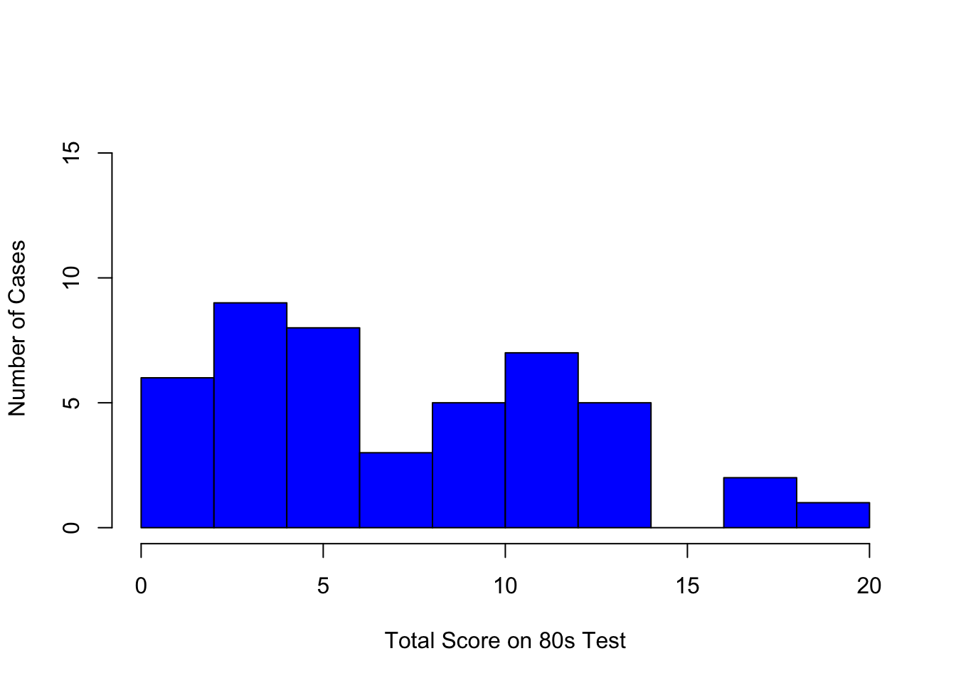
For this example I'm going to use data from a test I give to first year doctoral students in the University of Colorado's School of Education that attempts to measure the construct of 80s Music Fluency. I have data on 46 students who took my 20 item test. Each item consists of the first 30 seconds of a song that was a top 10 hit from the 1980s. An item is scored as correct (1) if the student can name the title of the song or the artist. Otherwise it is scored as incorrect (0).
```{r echo=FALSE}
data<-read.csv("80sresults_pilot_data_analysis.csv")
d <- data[,18:37]
total<-apply(d,1,sum)
hist(total,main=" ",xlab="Total Score on 80s Test"
,ylab="Number of Cases",ylim=c(0,16),col="blue")
```
Some descriptive stats for the total score on the test
```{r}
summary(total)
```
It should be clear that the 80s music fluency of my students left a lot to be desired!
How reliable are the scores from this test? What we want to know is this: How much of the total variability that we observe in 80s test performance, `r round(var(data$TOTAL),digits=1)`, is "true" variability? Let's investigate using what we've learned about reliability in general and $\alpha$ in particular.
### Using the function alpha in the R package psych
```{r warning=FALSE}
library("psych")
x<-alpha(d)
round(x$total$std.alpha,3)
round(x$total$raw_alpha,3)
round(x$total$average_r,3)
```
Let's start by looking at the overall results.
The alpha function returns three key statistics relevant to the presentation this far:
1. std.alpha = standardized alpha and is equivalent to equations 10 and 11 above when each item has been standardized to have a common variance of 1.
2. raw.alpha = alpha computed using equation 5 in DDLL, which is $\alpha=\frac{m\frac{\bar{c}}{s^2}}{1+\left(m-1\right)\frac{\bar{c}}{s^2}}$
3. average_r = average interitem correlation, $\bar{r}$
In this example, the std.alpha value is `r round(x$total$std.alpha,digits=3)` and the raw.alpha value is `r round(x$total$raw_alpha,digits=3)`. The average_r is `r round(x$total$average_r, digits=3)`.
We can also get item-specific information. The table below provides, for each item, the correlation between each item and the total score (both with and without the item included in the total score) as well and the mean (equivalent to proportion correct since these items are dichotomously scored) and sd for each item.
```{r}
round(x$item.stats[4:7],digits=3)
```
The alpha function also provides other information I'm not going to get into here, such as the impact on $\alpha$ if an item were dropped from the scale.
Let's go ahead and apply DDLL's equation 3 (my equation 11) above
$$\alpha=\frac{m\bar{r}}{1+(m-1)\bar{r}}$$
to show that it gives the same reliability estimate we get using the alpha function.
```{r}
m<-ncol(d)
rbar<-x$total$average_r
round(m*rbar/(1+(m-1)*rbar),3)
```
Same result!
Now let's see if we can "approximate" $\alpha$ using $\alpha \approx \frac{\bar{r}}{V}$. We already know $\bar{r}$, but we need to find $V$. In keeping with the definition of $V$, we need to extract the first principal component from the item correlation matrix and express this as a proportion of total variance.
```{r echo=TRUE,comment=""}
fpc<-principal(d,nfactors=1)
V<-fpc$values[1]/ncol(d)
round(V,3)
round(rbar/V,3)
```
So this is interesting, notice that we now have a value for $\alpha$ that is somewhat lower, at `r round(rbar/V,digits=3)`. But recall from equation 11 that this is just an approximation of $\alpha$, and as such it is still pretty close to what we get from direct application of equation 10.
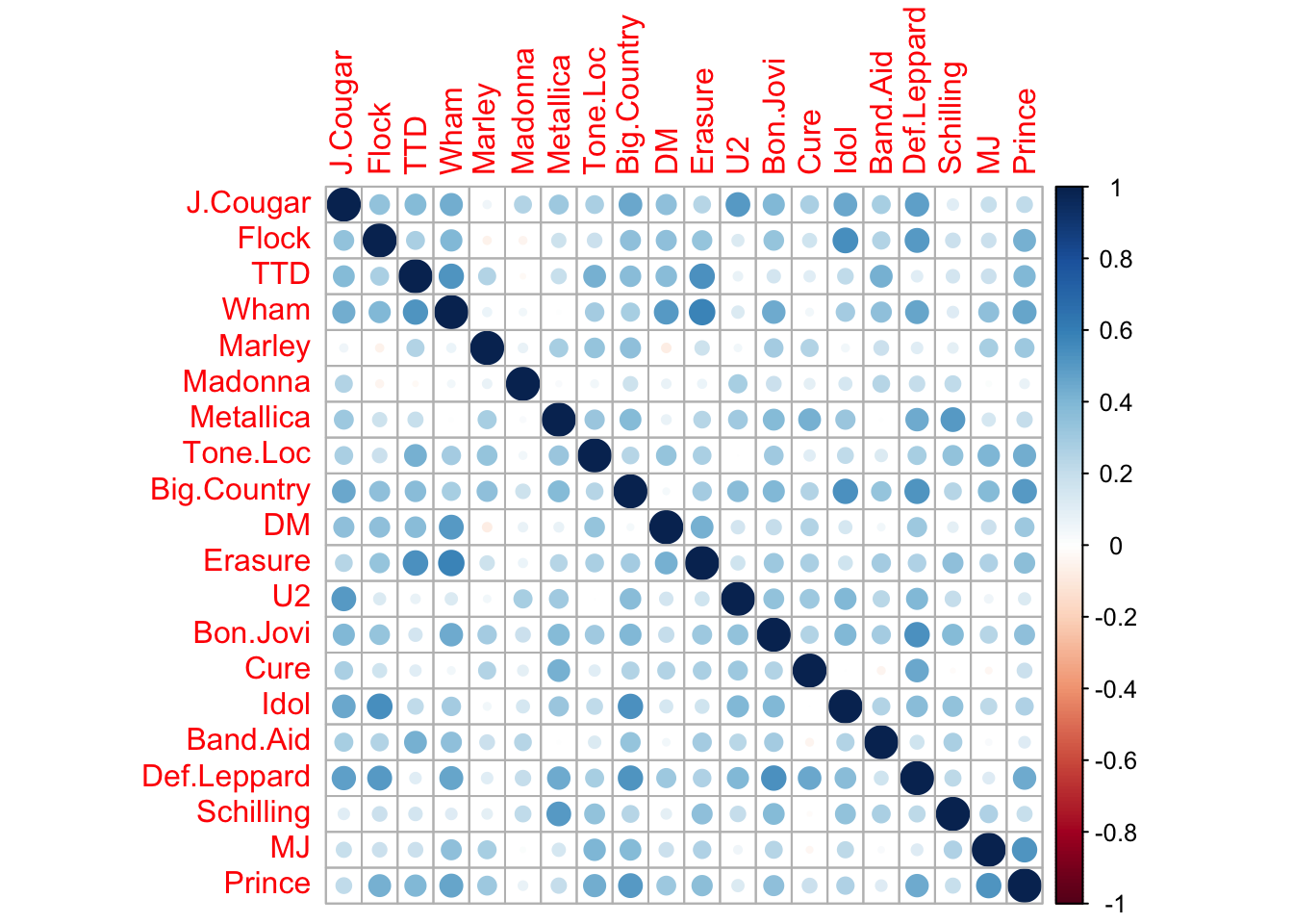
Let's have a closer look at the dimensionality of this 80s music test.
```{r}
library(corrplot)
corrplot(cor(d))
```
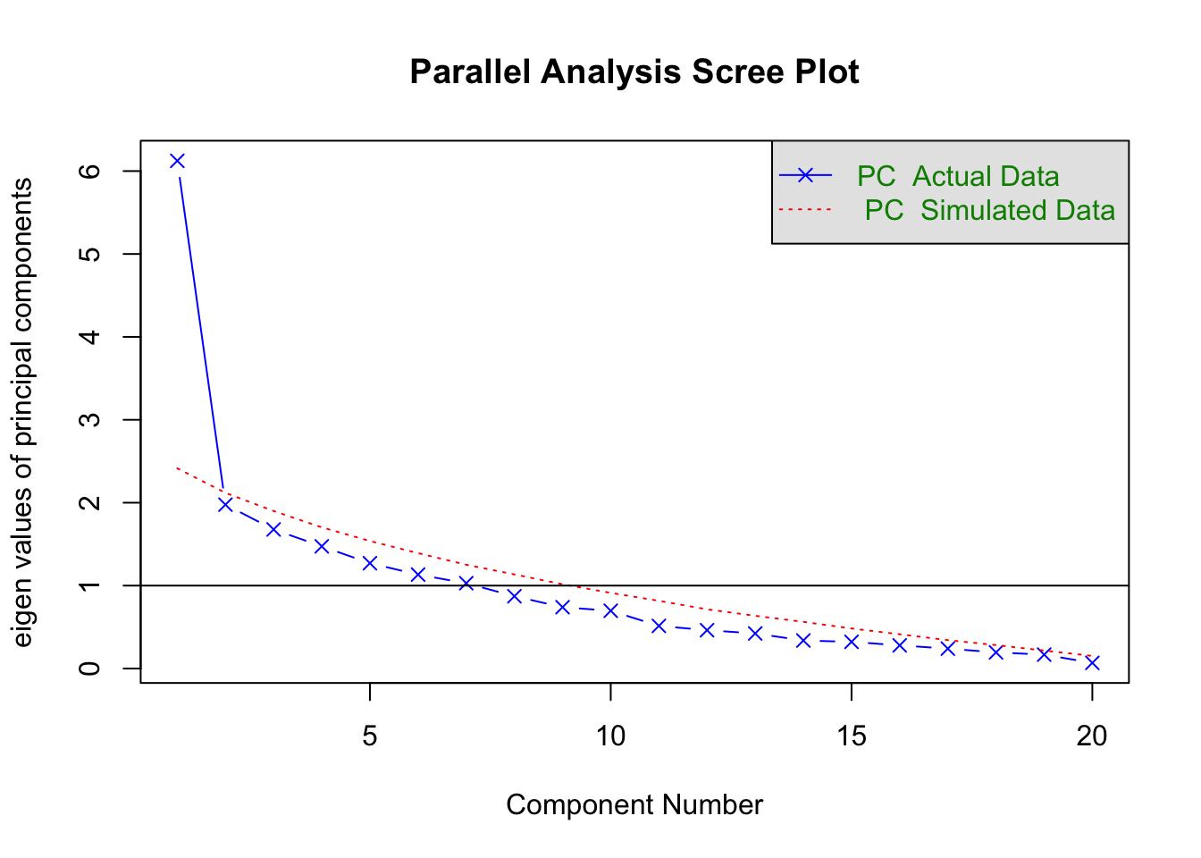
```{r}
cm<-cor(d)
fa.parallel(cm, n.obs = nrow(d),fm="pa", fa="pc",
       main = "Parallel Analysis Scree Plot",
        n.iter=100,error.bars=FALSE,ylabel=NULL,show.legend=TRUE)
```
The results seem to suggest we will do pretty well with a single factor solution.
# Alpha as a lower bound from a factor analytic standpoint
Note: This section gets a bit more technical than the sections above. Prior exposure to readings and coursework in factor analysis will help.
It's important to understand that $\alpha$, something we can compute, is not necessarily the same thing as $\rho_{XT}$. Instead, it is a _lower bound_ to $\rho_{XX^\prime}$. This means that $\alpha \leq \rho_{XX^\prime}$. For a proof that shows why $\alpha$ should be regarded as a lower bound, see Novick & Lewis (1967), pages 4-6. In fact, in their 1967 article, Novick & Lewis note that alpha is not necessarily even the best lower bound estimate. The first person to point this out and establish the concept of a "lower bound" for reliability was Louis Guttman, (see Guttman, 1945; 1953). It was in Guttman (1945) that he first derived what we are now calling Cronbach's alpha.
This raises an obvious question: when will $\alpha = \rho_{XX^\prime}$?
## Essential Tau Equivalence
To answer this question, Novick & Lewis (1967) first introduced the concept of *essential tau equivalence*. To express this mathematically, consider any two test items, $X_g$ and $X_h$. The items in each form have been sampled from the same universe of items eligible for inclusion on the test in question. For each item, we posit that the fundamental equation of classical test theory holds, so we can write $X_g = T_g + E_g$ and $X_h = T_h + E_h$. Now consider expressing the true score for one item as a linear function of the other:
$$T_g = a_{gh} + b_{gh}T_{h}$$
*If the two items are _tau equivalent_, $a_{gh}=0$ and $b_{gh}=1$.
*If the two item are _essentially tau equivalent_, $a_{gh}$ can vary but $b_{gh}=1$.
In other words, for tau equivalence to hold at the item level, it must be the case that all items have the same difficulty and the same intercorrelation.
Essential tau equivalence relaxes the assumption that pairs of items need to have the same difficulty, but does require them to have the same intercorrelation. When essential tau equivalence holds between all items on a test, the average correlation between items is the same thing as the correlation between *any* two items. When essential tau equivalence holds, $\alpha = \rho_{XX^\prime}$.

Of course, essential tau equivalence is a pretty restrictive assumption, but it is an assumption that is, in principle at least, testable through the specification of a confirmatory factor analysis (CFA) model, an approach favored by Green & Yang (2015) who show how $\alpha$ can be computed directly from the estimates of a one a factor CFA model with restrictions placed on all item loadings. In other words, this means a model in which there is a single factor and all items have the same loading on this factor.
Green & Yang present an equation (#10 on p. 15 of their 2015 article) that can be used to compute $\alpha$ following the specification and estimation of a one factor CFA with a common loading and items that have been standardized to have a variance of 1.
$$\tag{13}\rho_{XX^\prime} = \alpha = \frac{J^2\lambda^2}{\sigma^2_{X}}$$
where $J$ = number of test items, and $\lambda$ represents a common factor loading. The numerator = variance in test items caused by the common factor. Think of the $J$ by $J$ variance-covariance matrix. Under the assumption of essential tau equivalence, each element of this model-implied matrix is $\lambda^2$ because all items have the same intercorrelation. So total variance explained by the common factor is just ${J^2\lambda^2}$.
The denominator, $\sigma^2_{X}$ represents total variance of test scores. But we in taking a model-based approach we don't get an estimate for this by finding the variance of the observed total score after summing over the $J$ items. Instead, we get this from our specification of the factor analytic model, such that $\hat{\sigma}^2_X = J^2\lambda^2 + Je$, where $e=1-\lambda^2$.
## Continuing Empirical Example using CFA
Let's return to estimation of the reliability of our 80s test. Instead of estimating $\alpha$ using equation 10 and observed item scores, we can instead fit the essential tau equivalence model using the function cfa from the R package lavaan, and then compute equation 13.
One thing that complicates this approach is that factor analysis assumes that indicator variables have a continuous distribution, and that each variable has a linear relationship with one or more latent factors. Let's see what happens if we ignore this for our items and just conduct a 1-factor CFA using default maximum likelihood estimation. One preliminary step I'm going to take here is to standardize all the items.
```{r}
library("lavaan")
means<-apply(d,2,mean)
sd<-apply(d,2,sd)
d.std<-scale(d,center=means,scale=sd)
tau_mod <- '
general =~
lambda*J.Cougar + lambda*Flock +
lambda*TTD + lambda*Wham + lambda*Marley +
lambda*Madonna + lambda*Metallica +
lambda*Tone.Loc + lambda*Big.Country +
lambda*DM + lambda*Erasure +
lambda*U2 + lambda*Bon.Jovi + lambda*Cure +
lambda*Idol + lambda*Band.Aid + lambda*Def.Leppard +
lambda*Schilling +lambda*MJ + lambda*Prince'
taumod <- cfa(model = tau_mod, data = d.std, std.lv = TRUE)
out<-lavInspect(taumod,what="est")
parameterEstimates(taumod)[1:20,1:6]
round((fitmeasures(taumod)[c("chisq","df","pvalue","chisq.scaled",
"df.scaled","pvalue.scaled","cfi","gfi","tli","rmsea",
"rmsea.pvalue","srmr")]),3)
```
Applying eqn 13 to results:
```{r}
J<-ncol(d)
lambda<-out$lambda[1]
e<-1-lambda^2
rel<-(J^2*lambda^2)/((J^2*lambda^2)+J*e)
round(rel,3)
```
So we get about the same estimate for reliability as we did using Cronbach's alpha. If the model fits the data, we can say that this estimate is not a lower bound to $\rho_{XX^\prime}$, but is an unbiased estimate of it. But does the model fit the data? It doesn't look like it.
* The standardized mean residual is `r fitmeasures(taumod)["srmr"]`.
* The RMSEA is `r fitmeasures(taumod)["rmsea"]`.
* The CFI is `r fitmeasures(taumod)["cfi"]`.
## A Congeneric Model
We can relax the assumption of essential tau equivalence and specify instead what is know as a *congeneric model*. This allows both the intercept and slope to vary for each item, but still assumes a one factor solution.

```{r}
con_mod <- '
general =~
J.Cougar + Flock +TTD + Wham + Marley + Madonna +
Metallica + Tone.Loc + Big.Country + DM + Erasure +
U2 + Bon.Jovi + Cure + Idol + Band.Aid + Def.Leppard +
Schilling + MJ + Prince'
artists<-names(d)
conmod <- cfa(model = con_mod, data = d, ordered = artists
    ,estimator = "DWLS", se = "robust", test = "scaled.shifted", std.lv = TRUE)
parameterEstimates(conmod)[1:20,]
round((fitmeasures(conmod)[c("chisq","df","pvalue","chisq.scaled","df.scaled",
                             "pvalue.scaled","cfi","gfi","tli","rmsea",
                             "rmsea.pvalue","srmr")]),3)
```
Notice that this model shows evidence of better fit, but with this illustrative example we have to be careful about these sorts of interpetations given our very small sample. Notice that the SRMR is still extremely high.
*The improvement in standardized mean residual is `r fitmeasures(conmod)["srmr"]-fitmeasures(taumod)["srmr"]`.
*The improvement in RMSEA is `r fitmeasures(conmod)["rmsea"]-fitmeasures(taumod)["rmsea"]`.
*The improvement in CFI is `r fitmeasures(conmod)["cfi"]-fitmeasures(taumod)["cfi"]`.
To complete the example, having fit this model we can now use the more general formula Green & Yang provide for estimating reliability as the sum of item communalities over total item covariance (communalities + uniqueness). See equation 7 from Green & Yang.
```{r}
pe <- parameterestimates(conmod)
sumT <- sum(pe[1:15, "est"])^2
sume <- sum(pe[61:75, "est"])
sumX <- sumT+sume
round(sumT/sumX, 3)
```
So fitting the congeneric model doesn't significantly change the interpretation one gets about the reliability of these test scores.
# Summing Up: Takeaway Lessons
## 1. Reliability = consistency of results across replications of a measurement procedure
It's important to appreciate the difference between what people out in the world have in mind when they speak of reliability vs. the quantity that gets estimated using (most commonly) Cronbach's alpha. What people mean by reliability is that I will get very close to the same results if I step off and on a scale on my bathroom floor over and over again. What we need to check this are independent replications of the same measuring procedure. This is much harder to realize in educational and psychological measurement contexts.
## 2. A reliability coefficient is a means to an end
Classical Test Theory (CTT) was born from Charles Spearman's insight that when two variables have each been measured with error, the correlation between the two variables will be attenuated (weaker than it would have been if the variables were measured without error). Spearman derived a disattenuation formula that required estimates of each variable's reliability coefficient before it could be employed. That formula is
$$\rho(X,Y)=\frac{\rho(\hat{X},\hat{Y})}{\sqrt{{\sigma^2_{XT}}{\sigma^2_{YT}}}}$$
In addition, as test scores were increasingly being used to make inferences about individuals in the early 20th century, it became important to be able to report not just a person's test score, but their standard error of measurement (SEM). The SEM is a direct function of reliability:
$$SEM_X=\sqrt{1-\sigma^2_{XT}}*S_{X}$$
Notice that the two formulas above have a subtle difference from the versions I presented earlier. That is, here I use $\sigma^2_{XT}$ and $\sigma^2_{YT}$ instead of $\alpha_X$ and $\alpha_Y$. The former represent the statistical parameter of interest, the latter represent a specific approach taken to estimate the parameter of interest (i.e., Cronbach's alpha).
## 3. CTT depends on the premise of a within-person thought experiment
Originally, this was cast as follows: what would happen if we could administer the same test to the same person over and over again, brainwashing the person in between each testing to forget the previous testing experience? I have altered the thought experiment just slightly such that upon each replication the composition of the test itself can vary because it is comprised of a random sample of items from a universe of admissable items. But either way, the idea is that the observed distribution of scores would vary over replications, and the SD of this distribution would serve to quantify the uncertainty about each person's true score, defined as the average score across infinite replications. It is easy to lose sight of this thought experiment because the CTT model seems to focus attention on variability in test scores across people, not within each person. What we would really love to know is the standard error of measurement for each person: $\sigma_{e_j}$. This very likely is not the same value for each person!
## 4. The CTT population level model is $X = T + E$
There is no way to estimate $\sigma_{e_j}$ so we seek to estimate $\sigma_{E}$, where the latter represents the *average* of person-specific error variances for a defined population of test-takers. This is what brings us to the expression
$$\rho^2_{XT}=\frac{\sigma^2_{T}}{\sigma^2_{X}}$$
Remember that in the within-person thought experiment, it makes no sense to think of variability in true scores, as for each person the true score is a constant. It is only sensible to speak of this after have a sample or population of test-takers, each with their own true score.
## 5. The estimation of $\rho^2_{XT}$ depends on the availability of a parallel test
If you have two parallel versions of the same test, it can be shown that
$$\rho_{XX^\prime}=\frac{\sigma^2_{T}}{\sigma^2_{X}}$$
which, in words, means that the correlation between two parallel tests is equivalent to the proportion of observed score variance that is true score variance.
## 6. It is really hard to create and administer independent parallel tests
So what people tend to do instead is to look for parallel subtests within an existing test administration.
## 7. Cronbach's alpha is one popular way to estimate a reliability coefficient
It ultimately rests on the assumption that the set of items on a test can be conceptualized as a random sample from a universe of possible test items. If so, alpha gives an estimate of the average intercorrelation, corrected for restriction of range, that one can expect for randomly parallel tests. It is easy to compute.
$$ \alpha = \frac{m}{m-1} \left(1-\frac{\sum_{i=1}^{m}S^2_{X_i}}{S^2_{X}} \right) $$
## 8. It is really easy to misinterpret alpha
Alpha has a functional relationship with test length and item intercorrelations. So if it is high, this could either be because the test was long, the item intercorrelations are high, or some combination of the two. By itself it doesn't reveal whether a test is "internally consistent" and honestly, that concept itself is a bit vague. For alpha to give an unbiased estimate of the correlation we would get from two parallel tests, all the items on a test from which alpha is estimated need to have the same intercorrelation. So if this is what we mean by internally consistent, we should just check the correlation matrix of item responses, something best accomplished as part of a factor analysis. If internally consistent means that the correlations are high, that's a different thing to look for. Either way, you can't get this information just from looking at the value computed for alpha. It also doesn't indicate much about dimensionality (factor structure of a test).
## 9. Alpha is a lower bound estimate of reliability: consistency of rankings based on a test
Alpha provides a relatively conservative (lower bound) estimate of how consistent our ranking of individuals would be across replications of a test/survey procedure. It can be interpreted as an estimate of the proportion of observed score variance that is not attributable to chance error.
## 10. Error comes from facets of measurement that vary across replications and interact with the people taking the test
According to our within-person thought experiment, chance error comes from any facet in the procedure that could conceivably vary across replications and thereby interact with the ability of a person to answer a question correctly. But this ultimately depends upon how the investigator is conceptualizing the meaning of a replication. What stays fixed, what is random, and what is ignorable? Generalizability Theory was developed to articulate this more clearly.
# References
Cronbach, L. J. (1951). Coefficient alpha and the internal structure of tests. Psychometrika, 15, 297-334.
Cronbach, L. J., Gleser, G. C., Nanda, H., & Rajaratnam, N. (1972). The dependability of behavioral measurements: Theory of generalizability of scores and profiles. New York: John Wiley.
Davenport et al (2015) Reliability, dimensionality, and internal consistency as defined by Cronbach: Distinct albeit related concepts. Educational Measurement: Issues & Practice. Vol. 34, No. 4, pp. 4–9.
Davenport, E. C., Davison, M. L., Liou, P.-Y., & Love, Q. U. (2016). Easier said than done: Rejoinder on Sijtsma and on Green and Yang. Educational Measurement: Issues and Practice, 35(1), 6–10.
Friedman, S., & Weisberg, H. F. (1981). Interpreting the first eigenvalue of a correlation matrix. Educational and Psychological Measure- ment, 41, 11–21.
Guttman, L. (1945). A basis for analyzing test-retest reliability. Psychometrika, 10, 255-282.
Guttman, L. (1953). Reliability formulas that do not assume experimental independence. Psychometrika, 18, 225-239.
Green, S. & Yang, Y. (2015). Evaluation of dimensionality in the assessment of internal consistency reliability: Coefficient alpha and omega coefficients. Educational Measurement: Issues & Practice. Vol. 34, No. 4, pp. 14–20.
Novick, M. R., & Lewis, C. (1967). Coefficient alpha and the reliability of composite measurements. Psychometrika, 32(1), 1-13.
Sijtsma, K. (2015). Delimiting coefficient alpha from internal consistency and unidimensionality. Educational Measurement: Issues & Practice. Vol. 34, No. 4, pp. 10-13.
# Further Resources
Brennan, R. (2001). Generalizability Theory. New York: Springer-Verlag.
Green, S. B., Lissitz, R. W., & Mulaik, S. A. (1977). Limitations of coefficient alpha as an index of test unidimensionality. Educational and Psychological Measurement, 37, 827–838.
Sijtsma, K. (2009). On the use, the misuse, and the very limited usefulness of Cronbach’s alpha. Psychometrika, 74, 107–120.
Traub, R. & Rowly, G. (1991). Understanding Reliability. An NCME Instructional Module.
Wainer, H. and Thissen, D. (2001) True score theory: the traditional method. In Test Scoring, H. Wainer & D. Thissen (eds). Lawrence Erlbaum Associates. (Chapter 2, 23-71).