---
title: "Interpreting Item Characteristic Curves"
subtitle: "1PL, 2PL, and 3PL Models"
author: "Derek C. Briggs and Claude Code (Opus 4.6 & 4.7)"
output:
html_document:
toc: true
toc_float: true
code_folding: show
pdf_document:
toc: true
latex_engine: xelatex
---
```{r inject-rootdir, include=FALSE}
knitr::opts_knit$set(root.dir = "/Users/briggsd/Library/CloudStorage/Dropbox/Github/Measurement and Psychometrics/IRT Models for Dichotomously Scored Items/R Markdown Tutorials")
```
```{r setup, include=FALSE}
knitr::opts_chunk$set(echo = TRUE, message = FALSE, warning = FALSE)
```
## Introduction
This document covers the interpretation of Item Characteristic Curves (ICCs) for the 1PL (Rasch), 2PL, and 3PL IRT models for dichotomously scored items.
## Scores in CTT vs. IRT
| Classical Test Theory (CTT) | Item Response Theory (IRT) |
|:---------------------------|:---------------------------|
| Assumes $X = T + E$ | Uses response patterns to infer $\theta$ |
| Score = sum/average of responses | Score = estimated latent trait level |
| Assumes observed score is sufficient | Models probability of each response |
In IRT, we use the pattern of observed item responses to make an inference about the underlying latent trait level, $\theta$ ("theta").
Terms often used synonymously for $\theta$: construct, ability, proficiency, capability, attribute.
**Key property:** $\theta$ does not theoretically depend on the specific set of items written for any given test (but we use a specific set of item responses to measure it).
## Notation
| Symbol | Meaning |
|:-------|:--------|
| $X_{ip}$ | Response of person $p$ to item $i$ (0 or 1) |
| $\theta_p$ | Trait or ability level for person $p$ |
| $b_i$ | "Difficulty" or location of item $i$ |
| $a_i$ | Discrimination of item $i$ |
| $c_i$ | Lower asymptote ("guessing") for item $i$ |
| $P_i(\theta)$ | Probability of answering item $i$ correctly |
| $Q_i(\theta)$ | Probability of NOT answering correctly; $Q_i = 1 - P_i$ |
---
## The IRT Models
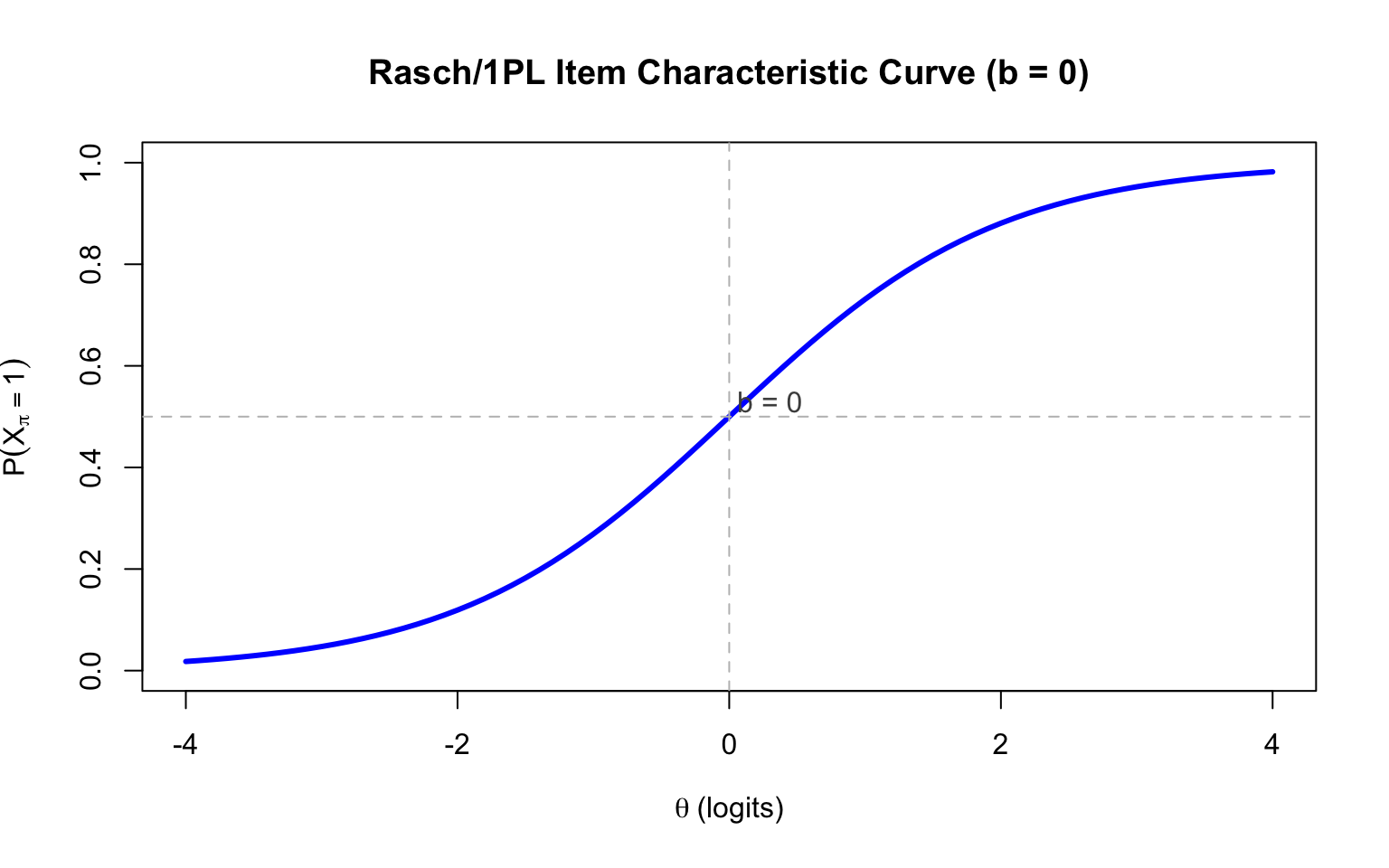
### The 1PL/Rasch Model
$$P(X_{pi} = 1 | \theta_p, b_i) = \frac{\exp(\theta_p - b_i)}{1 + \exp(\theta_p - b_i)}$$
- **One item parameter:** difficulty ($b_i$)
- $b_i$ is the point where $P(X_{pi} = 1) = 0.5$
- Assumes equal discrimination for all items
```{r rasch-icc, fig.width=8, fig.height=5}
# Function to calculate probability
calc_prob <- function(theta, a = 1, b = 0, c = 0) {
  c + (1 - c) * exp(a * (theta - b)) / (1 + exp(a * (theta - b)))
}

theta <- seq(-4, 4, 0.1)

# Plot Rasch ICC
plot(theta, calc_prob(theta, a = 1, b = 0), type = "l", lwd = 3, col = "blue",
     xlab = expression(theta ~ "(logits)"), ylab = expression(P(X[pi] == 1)),
     main = "Rasch/1PL Item Characteristic Curve (b = 0)",
     ylim = c(0, 1))
abline(h = 0.5, lty = 2, col = "gray")
abline(v = 0, lty = 2, col = "gray")
text(0.3, 0.53, "b = 0", col = "gray30")
```
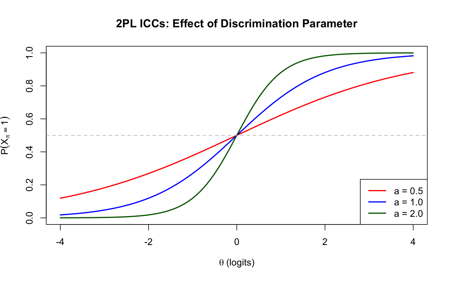
### The 2PL Model
$$P(X_{pi} = 1 | \theta_p, a_i, b_i) = \frac{\exp(a_i(\theta_p - b_i))}{1 + \exp(a_i(\theta_p - b_i))}$$
- **Two item parameters:** discrimination ($a_i$) and difficulty ($b_i$)
- $a_i$ controls the slope (steepness) of the ICC at $b_i$
- Higher $a_i$ = steeper slope = better discriminating item
```{r twopl-icc, fig.width=8, fig.height=5}
# Compare different discrimination values
plot(theta, calc_prob(theta, a = 0.5, b = 0), type = "l", lwd = 2, col = "red",
     xlab = expression(theta ~ "(logits)"), ylab = expression(P(X[pi] == 1)),
     main = "2PL ICCs: Effect of Discrimination Parameter",
     ylim = c(0, 1))
lines(theta, calc_prob(theta, a = 1, b = 0), lwd = 2, col = "blue")
lines(theta, calc_prob(theta, a = 2, b = 0), lwd = 2, col = "darkgreen")
abline(h = 0.5, lty = 2, col = "gray")
legend("bottomright", legend = c("a = 0.5", "a = 1.0", "a = 2.0"),
       col = c("red", "blue", "darkgreen"), lwd = 2)
```
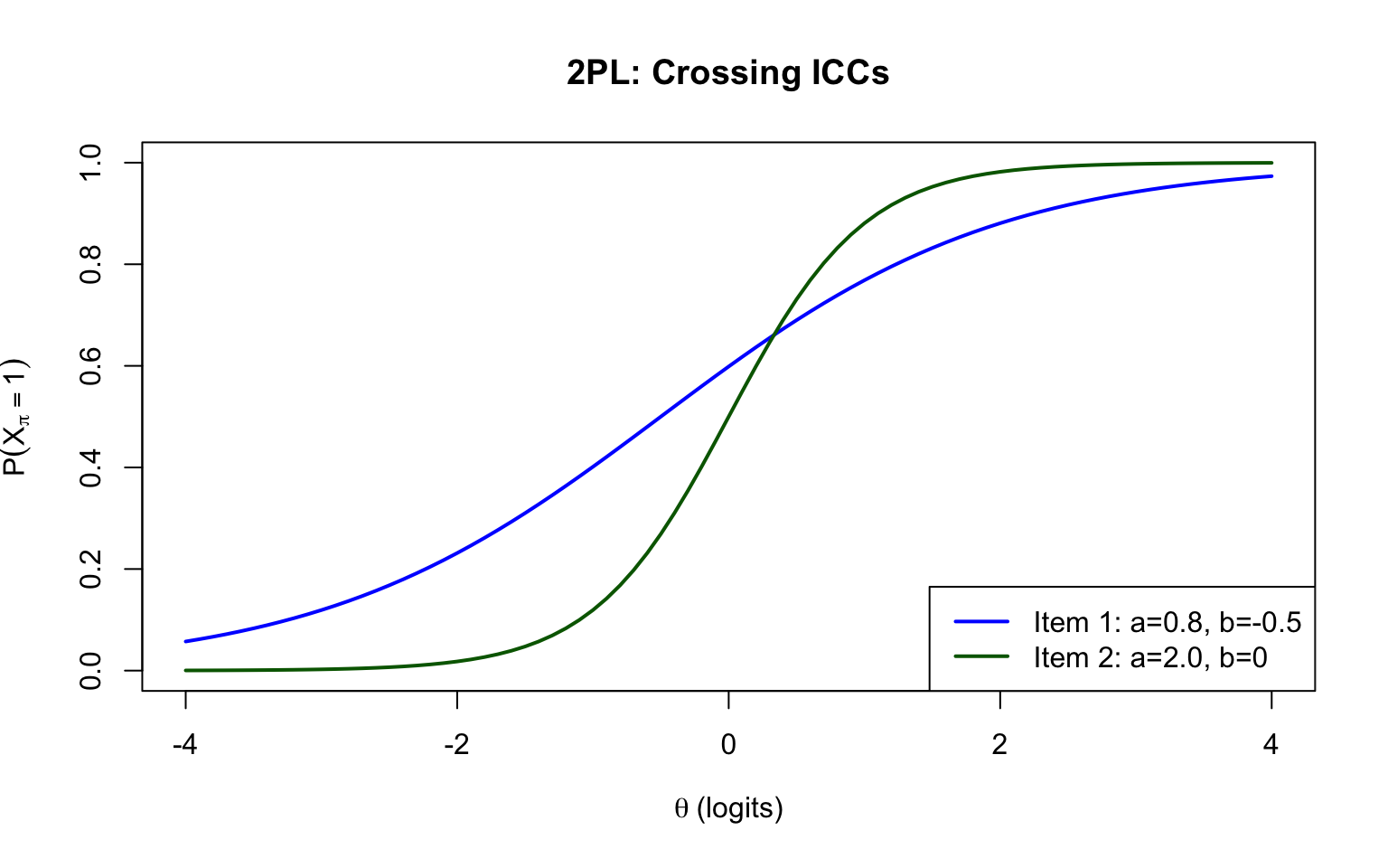
**Important:** In the 2PL model, different ICCs can cross. This means relative item difficulty can depend on the ability level of the test-taker.
```{r crossing-iccs, fig.width=8, fig.height=5}
plot(theta, calc_prob(theta, a = 0.8, b = -0.5), type = "l", lwd = 2, col = "blue",
     xlab = expression(theta ~ "(logits)"), ylab = expression(P(X[pi] == 1)),
     main = "2PL: Crossing ICCs",
     ylim = c(0, 1))
lines(theta, calc_prob(theta, a = 2, b = 0), lwd = 2, col = "darkgreen")
legend("bottomright", legend = c("Item 1: a=0.8, b=-0.5", "Item 2: a=2.0, b=0"),
       col = c("blue", "darkgreen"), lwd = 2)
```
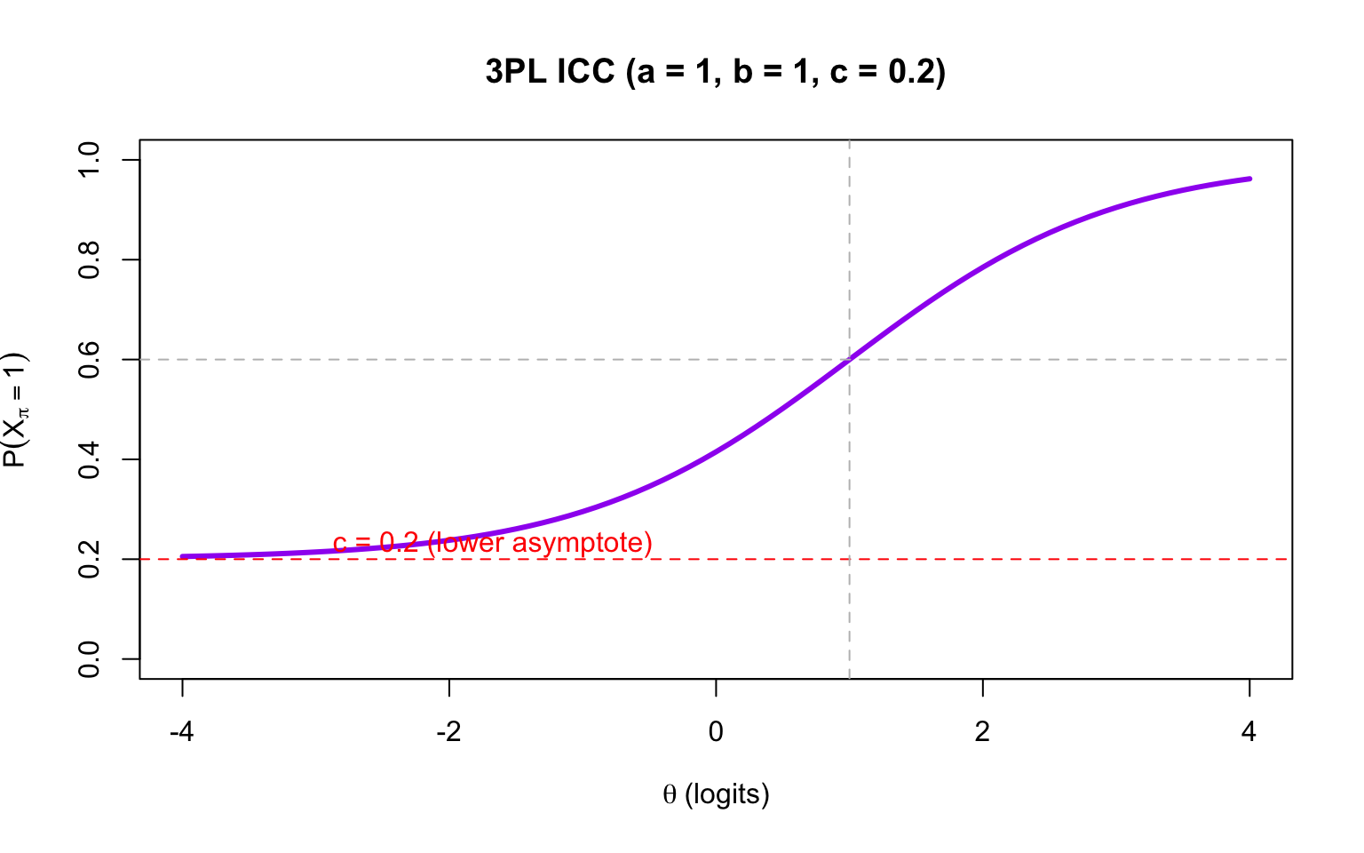
### The 3PL Model
$$P(X_{pi} = 1 | \theta_p, a_i, b_i, c_i) = c_i + (1 - c_i) \frac{\exp(a_i(\theta_p - b_i))}{1 + \exp(a_i(\theta_p - b_i))}$$
- **Three item parameters:** discrimination ($a_i$), difficulty ($b_i$), pseudo-guessing ($c_i$)
- $c_i$ is the lower asymptote (probability of correct response by guessing)
- **Note:** In the 3PL, $b_i$ is no longer the 50% point; it corresponds to $P = 0.5 + 0.5c_i$
```{r threepl-icc, fig.width=8, fig.height=5}
# 3PL ICC
plot(theta, calc_prob(theta, a = 1, b = 1, c = 0.2), type = "l", lwd = 3, col = "purple",
     xlab = expression(theta ~ "(logits)"), ylab = expression(P(X[pi] == 1)),
     main = "3PL ICC (a = 1, b = 1, c = 0.2)",
     ylim = c(0, 1))
abline(h = 0.2, lty = 2, col = "red")
abline(h = 0.6, lty = 2, col = "gray")  # 0.5 + 0.5*0.2 = 0.6
abline(v = 1, lty = 2, col = "gray")
text(-3, 0.23, "c = 0.2 (lower asymptote)", col = "red", pos = 4)
```
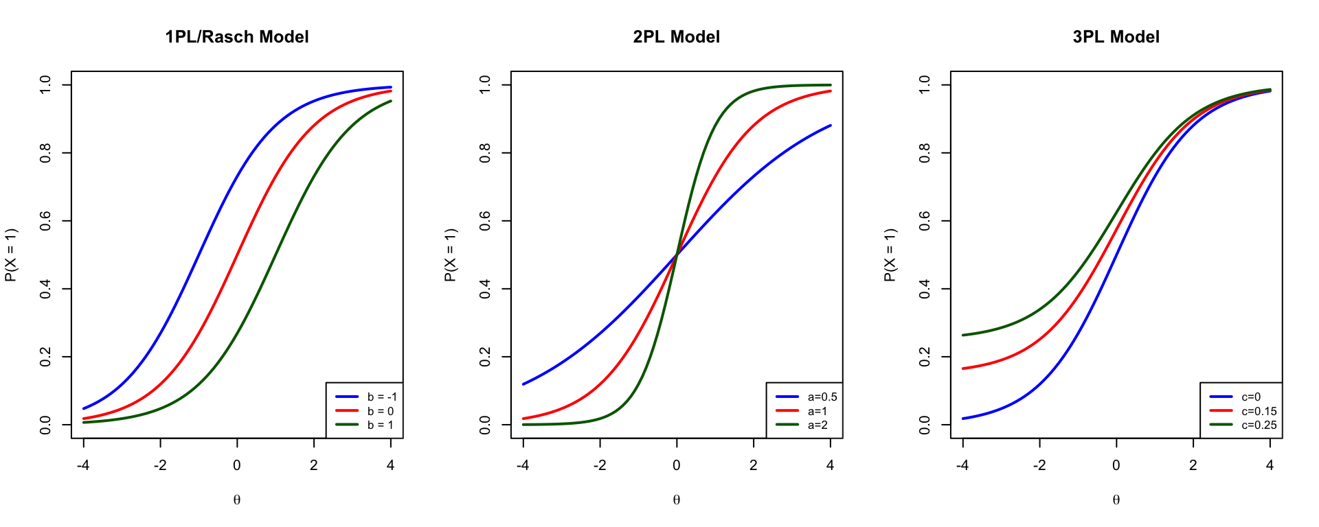
### Comparing All Three Models
```{r compare-models, fig.width=10, fig.height=4}
par(mfrow = c(1, 3))

# 1PL
b_vals <- c(-1, 0, 1)
plot(theta, calc_prob(theta, a = 1, b = b_vals[1]), type = "l", lwd = 2,
     col = "blue", xlab = expression(theta), ylab = "P(X = 1)",
     main = "1PL/Rasch Model", ylim = c(0, 1))
lines(theta, calc_prob(theta, a = 1, b = b_vals[2]), lwd = 2, col = "red")
lines(theta, calc_prob(theta, a = 1, b = b_vals[3]), lwd = 2, col = "darkgreen")
legend("bottomright", legend = paste("b =", b_vals), col = c("blue", "red", "darkgreen"), lwd = 2, cex = 0.8)

# 2PL
plot(theta, calc_prob(theta, a = 0.5, b = 0), type = "l", lwd = 2,
     col = "blue", xlab = expression(theta), ylab = "P(X = 1)",
     main = "2PL Model", ylim = c(0, 1))
lines(theta, calc_prob(theta, a = 1, b = 0), lwd = 2, col = "red")
lines(theta, calc_prob(theta, a = 2, b = 0), lwd = 2, col = "darkgreen")
legend("bottomright", legend = c("a=0.5", "a=1", "a=2"), col = c("blue", "red", "darkgreen"), lwd = 2, cex = 0.8)

# 3PL
plot(theta, calc_prob(theta, a = 1, b = 0, c = 0), type = "l", lwd = 2,
     col = "blue", xlab = expression(theta), ylab = "P(X = 1)",
     main = "3PL Model", ylim = c(0, 1))
lines(theta, calc_prob(theta, a = 1, b = 0, c = 0.15), lwd = 2, col = "red")
lines(theta, calc_prob(theta, a = 1, b = 0, c = 0.25), lwd = 2, col = "darkgreen")
legend("bottomright", legend = c("c=0", "c=0.15", "c=0.25"), col = c("blue", "red", "darkgreen"), lwd = 2, cex = 0.8)
par(mfrow = c(1, 1))
```
---
## Logits and Alternative Forms
The units of $\theta$, $b$, and $a$ are **logit** values. The $c$ parameter is on the probability scale.
For the 1PL and 2PL, we can show that:
$$\ln\left(\frac{P(X_{pi} = 1)}{1 - P(X_{pi} = 1)}\right) = a_i(\theta_p - b_i)$$
### Slope-Intercept Form
Sometimes you'll see the models written in slope-intercept form:
$$P(X_{pi} = 1) = c_i + (1 - c_i) \frac{\exp(a_i\theta_p + d_i)}{1 + \exp(a_i\theta_p + d_i)}$$
where $d_i = -a_i \cdot b_i$ (or equivalently, $b_i = -d_i / a_i$).
Many IRT programs estimate $d_i$ and then convert to $b_i$.
---
## Activity: Three-Item Test
Consider a test with three items with the following parameters:
```{r item-params}
items <- data.frame(
  Item = 1:3,
  a = c(1, 1, 2),
  b = c(-1.5, 0, 0.2),
  c = c(0.2, 0.2, 0.3)
)
knitr::kable(items, caption = "Item Parameters for Three-Item Test")
```
### Visualizing the ICCs
```{r three-item-plot, fig.width=8, fig.height=6}
theta <- seq(-4, 4, 0.1)

# Calculate probabilities for each item
p1 <- calc_prob(theta, a = 1, b = -1.5, c = 0.2)
p2 <- calc_prob(theta, a = 1, b = 0, c = 0.2)
p3 <- calc_prob(theta, a = 2, b = 0.2, c = 0.3)

plot(theta, p1, type = "l", lwd = 3, col = "blue",
     xlab = expression(theta), ylab = expression(P(X[i] == 1)),
     main = "ICCs for Three-Item Test",
     ylim = c(0, 1))
lines(theta, p2, lwd = 3, col = "red")
lines(theta, p3, lwd = 3, col = "darkgreen")
legend("bottomright",
       legend = c("Item 1: a=1, b=-1.5, c=0.2",
                  "Item 2: a=1, b=0, c=0.2",
                  "Item 3: a=2, b=0.2, c=0.3"),
       col = c("blue", "red", "darkgreen"), lwd = 3)
```
### Practice Questions
1. **Compare the difficulty of Item 1 vs. Item 2**
- Items 1 and 2 have the same discrimination ($a = 1$) and guessing ($c = 0.2$)
- Item 1 has $b = -1.5$, Item 2 has $b = 0$
- Item 1 is **easier** (lower b = easier)
2. **Compare the difficulty of Item 2 vs. Item 3**
- Different discrimination and guessing parameters make this more complex
- The ICCs cross, so relative difficulty depends on $\theta$
3. **Calculate response vector probabilities**
```{r response-probs}
# Function to calculate probability of response vector
calc_vector_prob <- function(theta, responses, a, b, c) {
  prob <- 1
  for (i in 1:length(responses)) {
    p_i <- calc_prob(theta, a[i], b[i], c[i])
    if (responses[i] == 1) {
      prob <- prob * p_i
    } else {
      prob <- prob * (1 - p_i)
    }
  }
  return(prob)
}

# Item parameters
a <- c(1, 1, 2)
b <- c(-1.5, 0, 0.2)
c <- c(0.2, 0.2, 0.3)

# Theta values
theta_vals <- c(-4.0, -1.1, 0, 1.6)

# Response patterns
patterns <- list(c(0, 0, 0), c(0, 1, 0), c(1, 1, 1))
pattern_names <- c("000", "010", "111")

# Calculate probabilities
results <- matrix(NA, nrow = length(theta_vals), ncol = length(patterns))
for (i in 1:length(theta_vals)) {
  for (j in 1:length(patterns)) {
    results[i, j] <- calc_vector_prob(theta_vals[i], patterns[[j]], a, b, c)
  }
}

results_df <- data.frame(
  Theta = theta_vals,
  `000` = round(results[, 1], 3),
  `010` = round(results[, 2], 3),
  `111` = round(results[, 3], 3),
  check.names = FALSE
)

knitr::kable(results_df, caption = "Probability of Each Response Vector by Theta")
```
**Interpretation:**
- At $\theta = -4.0$: The "000" pattern (all wrong) is most likely
- At $\theta = 1.6$: The "111" pattern (all correct) is most likely
- The "010" pattern (only item 2 correct) has relatively low probability at all theta levels
---
## Fitting IRT Models with mirt
Now let's use the `mirt` package in R to fit IRT models to real data.
```{r load-mirt}
library(mirt)
```
### Load and Prepare Data
```{r load-data}
forma <- read.csv("../Data/pset1_formA.csv")
forma <- forma[, 1:15]  # Use first 15 items
```
### Fit 1PL, 2PL, and 3PL Models
```{r fit-models, results='hide'}
# Fit the models
mirt_1pl <- mirt(forma, model = 1, itemtype = "Rasch", method = "EM")
mirt_2pl <- mirt(forma, model = 1, itemtype = "2PL", method = "EM")
mirt_3pl <- mirt(forma, model = 1, itemtype = "3PL", method = "EM")
```
### Extract and Compare Parameters
```{r compare-params}
# Extract coefficients in IRT parameterization
coef_1pl <- coef(mirt_1pl, simplify = TRUE, IRTpars = TRUE)
coef_2pl <- coef(mirt_2pl, simplify = TRUE, IRTpars = TRUE)
coef_3pl <- coef(mirt_3pl, simplify = TRUE, IRTpars = TRUE)

# Create comparison table
comparison <- data.frame(
  Item = rownames(coef_2pl$items),
  a_1PL = round(coef_1pl$items[, 1], 3),
  b_1PL = round(coef_1pl$items[, 2], 3),
  a_2PL = round(coef_2pl$items[, 1], 3),
  b_2PL = round(coef_2pl$items[, 2], 3),
  a_3PL = round(coef_3pl$items[, 1], 3),
  b_3PL = round(coef_3pl$items[, 2], 3),
  c_3PL = round(coef_3pl$items[, 3], 3)
)

knitr::kable(comparison, caption = "Parameter Estimates Across Models")
```
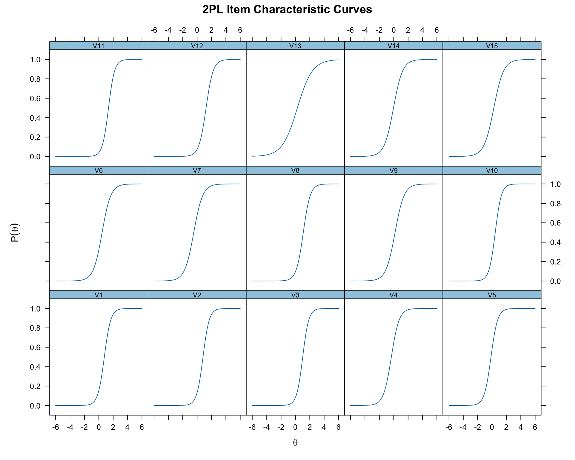
### Plot ICCs
```{r plot-iccs, fig.width=10, fig.height=8}
# Plot ICCs for 2PL model
plot(mirt_2pl, type = 'trace', main = "2PL Item Characteristic Curves")
```
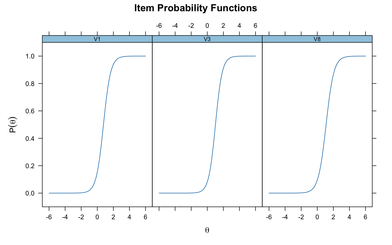
### Plot Specific Items
```{r specific-items, fig.width=8, fig.height=5}
# Compare specific items
plot(mirt_2pl, which.items = c(1, 3, 8), type = 'trace')
```
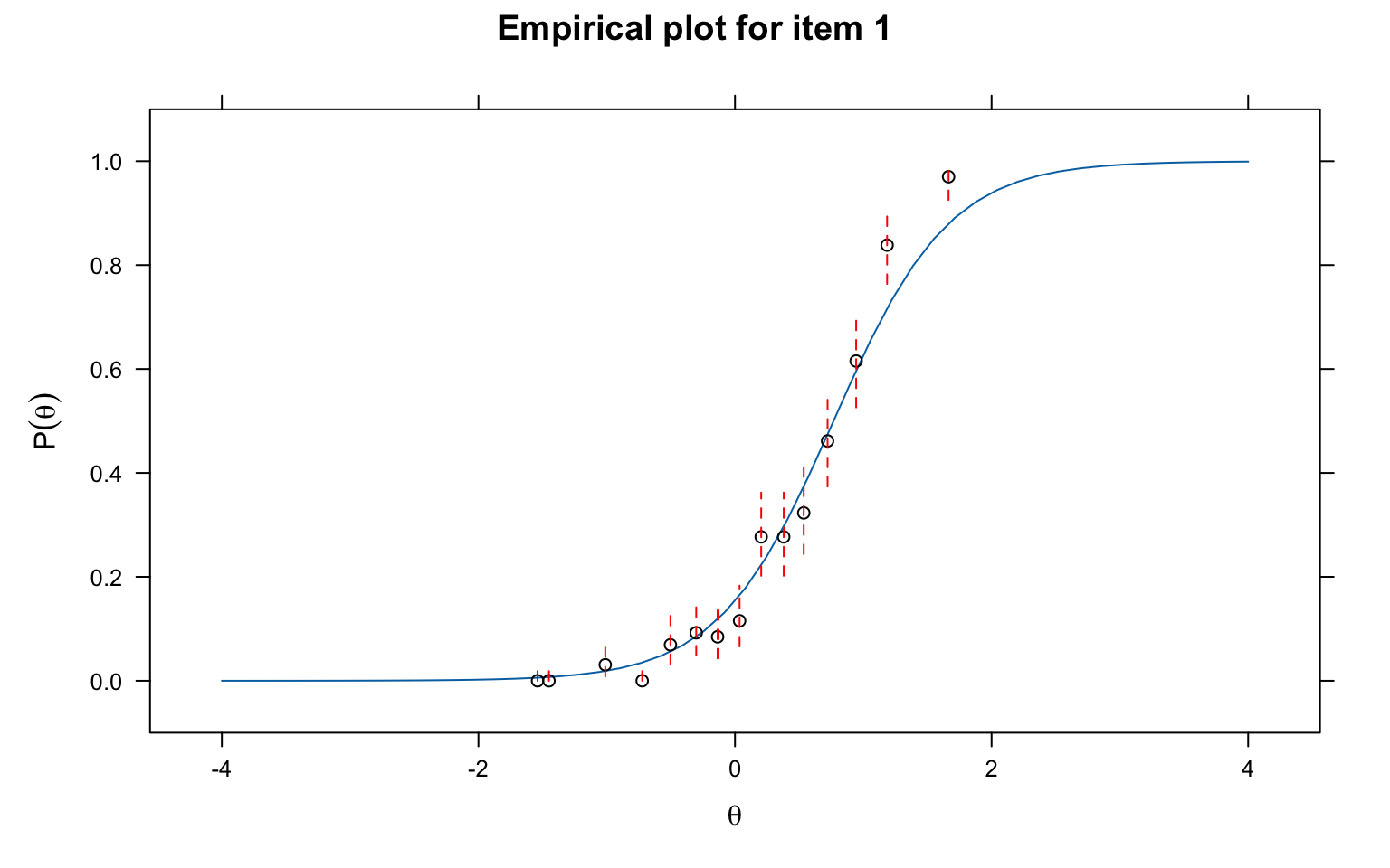
### Check Item Fit
```{r item-fit, fig.width=8, fig.height=5}
# Observed vs. predicted for Item 1
itemfit(mirt_2pl, group.bins = 15, empirical.plot = 1)
```
---
## Summary
1. The **1PL/Rasch model** has one item parameter (difficulty) and assumes equal discrimination
2. The **2PL model** adds a discrimination parameter, allowing ICCs to have different slopes
3. The **3PL model** adds a lower asymptote (guessing) parameter
4. In the 2PL and 3PL, ICCs can cross, meaning relative item difficulty may depend on ability level
5. The `mirt` package provides a flexible framework for fitting these models in R
---
## Interactive Practice
For an interactive version of the three-item test activity, see the **Shiny app** in the `Shiny Apps` folder.