14  IRT Models for Polytomously Scored Items

EDUC 8720

15 Introduction

15.1 What Are Polytomous Items?

The IRT models we have examined so far have been designed for dichotomously scored items—items with exactly two scored outcomes (e.g., correct/incorrect). Many assessment contexts, however, involve polytomous items: items scored into three or more categories. Examples include:

• Likert scales: Strongly Disagree / Disagree / Agree / Strongly Agree
• Partial credit tasks: Constructed response items with multiple score points (0, 1, 2, 3)
• Rating scales: Performance ratings (e.g., Fail / Pass / Credit / Distinction)

A fundamental question is whether the response categories are ordinal (ordered in terms of the trait) or nominal (unordered, distinct options). This distinction determines which family of polytomous IRT model is appropriate.

15.2 Two Families of Models

Mellenbergh (1995) provided a useful taxonomy of polytomous IRT models based on how they relate category probabilities to the latent trait:

1. Adjacent-category models: The model is built from the ratio of probabilities of responding in adjacent categories (e.g., category \(k\) vs. category \(k+1\)). These are sometimes called “divide-by-total” models (Thissen & Steinberg, 1986). This family includes the Partial Credit Model (PCM), Generalized Partial Credit Model (GPCM), and Rating Scale Model (RSM).

2. Cumulative models: The model is built from the cumulative probability of responding at or above a given category. This family includes the Graded Response Model (GRM).

3. Nominal models: No assumed ordering of categories. The Nominal Response Model (NRM) falls here.

15.3 Historical Context

The key polytomous IRT models were developed over a 25-year span:

Year	Model	Developer
1969	Graded Response Model (GRM)	Fumiko Samejima
1972	Nominal Response Model (NRM)	R. Darrell Bock
1978	Rating Scale Model (RSM)	David Andrich
1982	Partial Credit Model (PCM)	Geoff Masters
1992	Generalized Partial Credit Model (GPCM)	Eiji Muraki

In this tutorial we will present these models in an order that emphasizes their conceptual relationships: PCM → GPCM → RSM → GRM → NRM.

15.4 Key References

• Andrich, D. (1978). A rating formulation for ordered response categories. Psychometrika, 43, 561–573.
• Andrich, D. (2015). The problem with the step metaphor for polytomous models for ordinal assessments. Educational Measurement: Issues and Practice, 34(2), 8–14.
• Embretson, S. E., & Reise, S. P. (2000). Item response theory for psychologists. Chapter 5.
• Penfield, R. D. (2014). An NCME instructional module on polytomous item response theory models. Educational Measurement: Issues and Practice, 33(1), 36–48.

16 The Verbal Aggression Data

16.1 Setup

library(mirt)
library(psych)

16.2 Data Description

We use the Verbal Aggression dataset, which has been widely used in IRT textbooks and articles (e.g., de Boeck & Wilson, 2004). The data come from a study of \(N = 316\) Belgian undergraduate students who rated their reactions to frustrating situations.

Each item is a combination of three facets:

• Situation (4 levels): A bus fails to stop for me (bus), I miss a train because a clerk gave me faulty information (train), the grocery store closes just as I am about to enter (store), the operator disconnects me when I had used up my last 10 cents for a call (call)
• Behavior mode (2 levels): want to do vs. actually do
• Behavior type (3 levels): curse, scold, shout

This creates \(4 \times 2 \times 3 = 24\) items. Items are scored: 0 = no, 1 = perhaps, 2 = yes.

The two “other to blame” situations (bus, train) might be expected to elicit more verbal aggression than the two “self to blame” situations (store, call). Similarly, “want to” items should generally be easier to endorse than “do” items.

d <- read.csv("verbagg_wide.csv")
cat("Dimensions:", nrow(d), "respondents x", ncol(d), "items\n")

Dimensions: 316 respondents x 24 items

16.3 Item Structure

# Create a reference table for the 24 items
item_info <- data.frame(
  Item = 1:24,
  Name = names(d),
  Situation = rep(c("bus", "train", "store", "call"), each = 6),
  Blame = rep(c("other", "other", "self", "self"), each = 6),
  Mode = rep(c("want", "do"), 12),
  Type = rep(rep(c("curse", "scold", "shout"), each = 2), 4)
)
knitr::kable(item_info, caption = "Structure of the 24 Verbal Aggression Items")

Structure of the 24 Verbal Aggression Items

Item	Name	Situation	Blame	Mode	Type
1	i1_bus_want_curse	bus	other	want	curse
2	i2_bus_do_curse	bus	other	do	curse
3	i3_bus_want_scold	bus	other	want	scold
4	i4_bus_do_scold	bus	other	do	scold
5	i5_bus_want_shout	bus	other	want	shout
6	i6_bus_do_shout	bus	other	do	shout
7	i7_train_want_curse	train	other	want	curse
8	i8_train_do_curse	train	other	do	curse
9	i9_train_want_scold	train	other	want	scold
10	i10_train_do_scold	train	other	do	scold
11	i11_train_want_shout	train	other	want	shout
12	i12_train_do_shout	train	other	do	shout
13	i13_store_want_curse	store	self	want	curse
14	i14_store_do_curse	store	self	do	curse
15	i15_store_want_scold	store	self	want	scold
16	i16_store_do_scold	store	self	do	scold
17	i17_store_want_shout	store	self	want	shout
18	i18_store_do_shout	store	self	do	shout
19	i19_call_want_curse	call	self	want	curse
20	i20_call_do_curse	call	self	do	curse
21	i21_call_want_scold	call	self	want	scold
22	i22_call_do_scold	call	self	do	scold
23	i23_call_want_shout	call	self	want	shout
24	i24_call_do_shout	call	self	do	shout

16.4 Motivating Questions

As we fit different models to these data, we will return to these substantive questions:

1. Which items require the most verbal aggression to endorse with a “yes” response?
2. How big are the distances between category thresholds (no/perhaps and perhaps/yes) for “want” items vs. “do” items?
3. How much more likely is verbal aggression in an “other to blame” vs. a “self to blame” scenario?
4. How do the answers to these questions change depending on which model we use?

16.5 Descriptive Statistics

# Response category frequencies for each item
cat_freq <- apply(d, 2, function(x) table(factor(x, levels = 0:2)))
cat_freq_df <- as.data.frame(t(cat_freq))
names(cat_freq_df) <- c("No (0)", "Perhaps (1)", "Yes (2)")
cat_freq_df$Item <- 1:24
cat_freq_df$Name <- names(d)
cat_freq_df <- cat_freq_df[, c("Item", "Name", "No (0)", "Perhaps (1)", "Yes (2)")]
knitr::kable(cat_freq_df, caption = "Response Category Frequencies by Item", row.names = FALSE)

Response Category Frequencies by Item

Item	Name	No (0)	Perhaps (1)	Yes (2)
1	i1_bus_want_curse	91	95	130
2	i2_bus_do_curse	91	108	117
3	i3_bus_want_scold	126	86	104
4	i4_bus_do_scold	136	97	83
5	i5_bus_want_shout	154	99	63
6	i6_bus_do_shout	208	68	40
7	i7_train_want_curse	67	112	137
8	i8_train_do_curse	109	97	110
9	i9_train_want_scold	118	93	105
10	i10_train_do_scold	162	92	62
11	i11_train_want_shout	158	84	74
12	i12_train_do_shout	238	53	25
13	i13_store_want_curse	128	120	68
14	i14_store_do_curse	171	108	37
15	i15_store_want_scold	198	90	28
16	i16_store_do_scold	239	61	16
17	i17_store_want_shout	240	63	13
18	i18_store_do_shout	287	25	4
19	i19_call_want_curse	98	127	91
20	i20_call_do_curse	118	117	81
21	i21_call_want_scold	179	88	49
22	i22_call_do_scold	181	91	44
23	i23_call_want_shout	217	64	35
24	i24_call_do_shout	259	43	14

# Total score distribution
tot <- rowSums(d)

hist(tot, breaks = seq(-0.5, max(tot) + 0.5, 1), las = 1, col = "steelblue",
     main = "Distribution of Total Scores", xlab = "Total Score (0–48)",
     ylab = "Frequency", border = "white")
abline(v = mean(tot), col = "red", lwd = 2, lty = 2)
legend("topright", legend = paste("Mean =", round(mean(tot), 1)),
       col = "red", lty = 2, lwd = 2, bty = "n")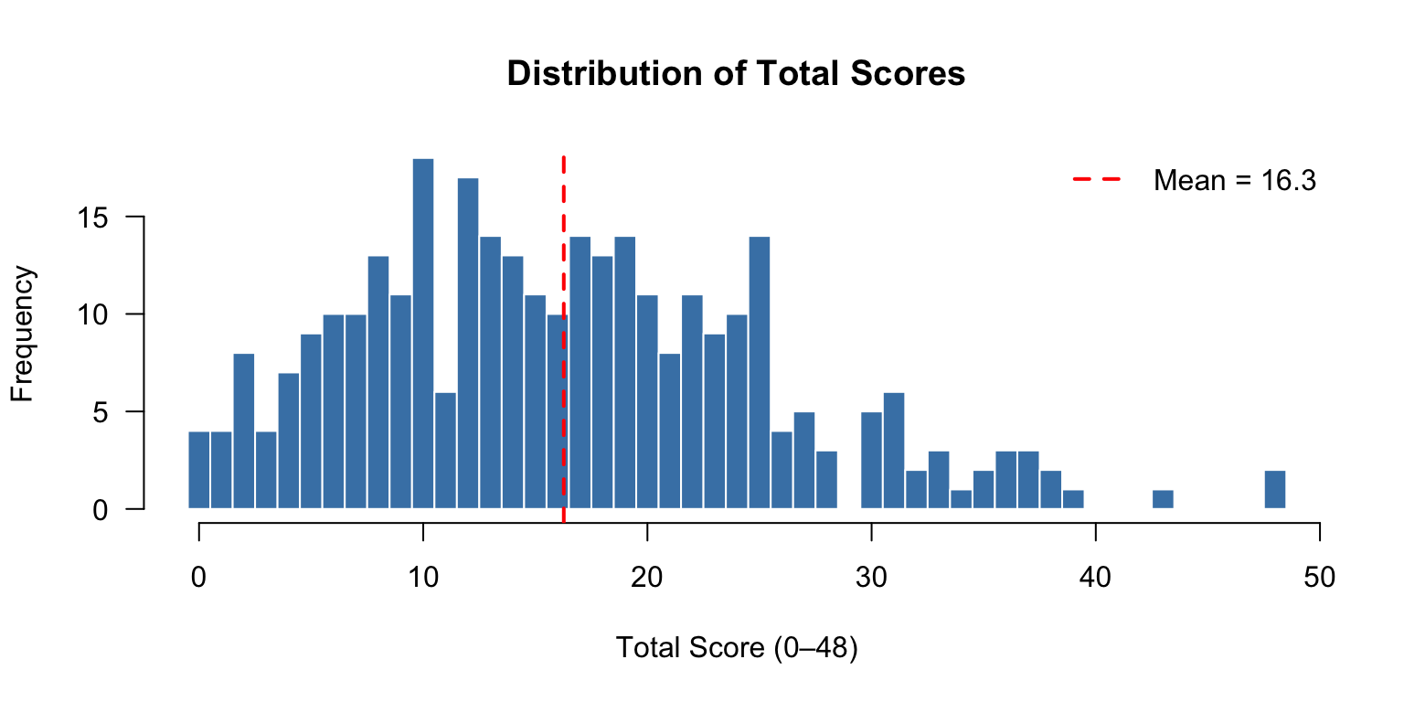

# Item means (analogous to classical difficulty)
item_means <- colMeans(d)

barplot(item_means, names.arg = 1:24, las = 1, col = "steelblue",
        main = "Item Means (Higher = More Verbal Aggression Endorsed)",
        xlab = "Item", ylab = "Mean Score (0–2)", ylim = c(0, 2),
        border = "white")

# Add reference lines for want vs. do
abline(h = mean(item_means[item_info$Mode == "want"]), col = "red", lty = 2)
abline(h = mean(item_means[item_info$Mode == "do"]), col = "blue", lty = 2)
legend("topright", legend = c("Mean: Want items", "Mean: Do items"),
       col = c("red", "blue"), lty = 2, lwd = 1.5, bty = "n", cex = 0.8)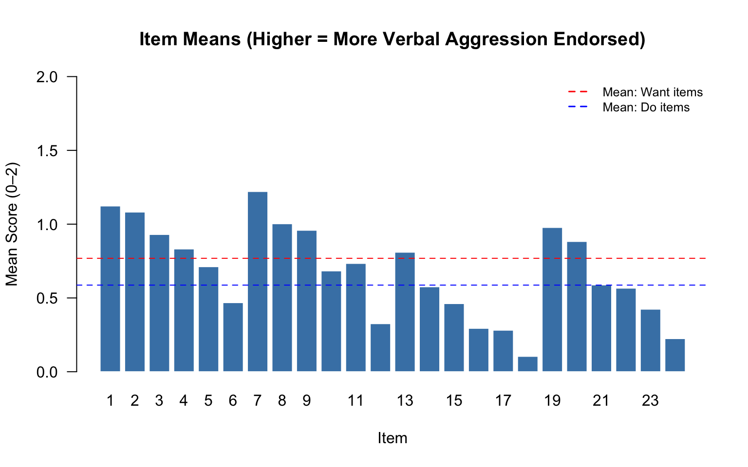

17 Checking Assumptions

17.1 Unidimensionality

Before fitting any IRT model, we should check the assumption that a single latent trait underlies the item responses.

fa.parallel(d, n.obs = nrow(d), fm = "minres", fa = "fa",
            main = "Parallel Analysis Scree Plot",
            n.iter = 100, error.bars = FALSE, SMC = FALSE,
            ylabel = NULL, show.legend = TRUE)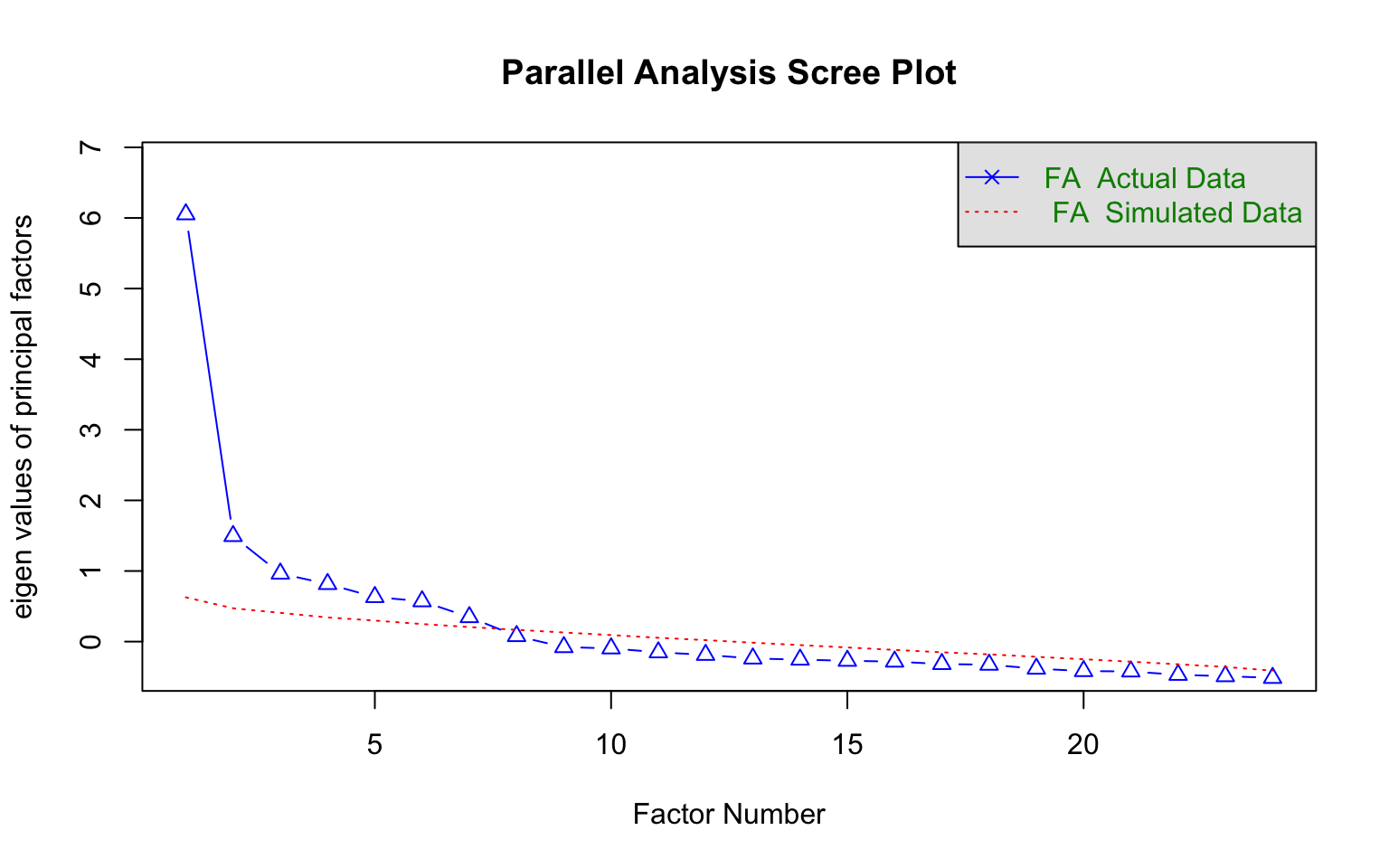

Parallel analysis suggests that the number of factors =  7  and the number of components =  NA 

The parallel analysis provides a screen for how many factors are supported by the data. For polytomous IRT models to be appropriate, we need evidence of a dominant first factor. A large gap between the first eigenvalue and the rest (and the parallel analysis reference line) supports the unidimensionality assumption.

# Check that all categories are used for each item
min_freq <- apply(d, 2, function(x) min(table(factor(x, levels = 0:2))))
cat("Minimum category frequency across items:", min(min_freq), "\n")

Minimum category frequency across items: 4 

cat("Items where minimum category count < 20:",
    paste(which(min_freq < 20), collapse = ", "), "\n")

Items where minimum category count < 20: 16, 17, 18, 24 

18 Partial Credit Model (PCM)

18.1 Model Overview

The Partial Credit Model (Masters, 1982) is a Rasch-family model for ordered polytomous responses. For an item with \(m+1\) response categories (scored \(0, 1, \ldots, m\)), the PCM specifies:

\[P(X_{ij} = k \mid \theta_j) = \frac{\exp\left(\sum_{v=0}^{k}(\theta_j - b_{iv})\right)}{\sum_{r=0}^{m}\exp\left(\sum_{v=0}^{r}(\theta_j - b_{iv})\right)}\]

where \(b_{iv}\) are the Andrich threshold parameters (with \(b_{i0} \equiv 0\) by convention). Each item has \(m\) threshold parameters that indicate the points on the trait continuum where adjacent categories are equally likely.

Key properties of the PCM:

• No discrimination parameter: All items are assumed to discriminate equally (as in the Rasch model for dichotomous items).
• Sufficient statistics: The total score is a sufficient statistic for \(\theta\).
• Item-specific thresholds: Each item can have its own set of threshold locations and distances between thresholds.

18.2 Fitting the PCM

pcm <- mirt(d, 1, itemtype = "Rasch")

18.3 Parameter Estimates

pcm_pars <- coef(pcm, IRTpars = TRUE, simplify = TRUE)$items
colnames(pcm_pars) <- c("a", "b1", "b2")
knitr::kable(round(pcm_pars, 3),
             caption = "PCM Parameter Estimates (Andrich Thresholds)")

PCM Parameter Estimates (Andrich Thresholds)

	a	b1	b2
i1_bus_want_curse	1	-0.421	-0.085
i2_bus_do_curse	1	-0.529	0.177
i3_bus_want_scold	1	0.130	0.151
i4_bus_do_scold	1	0.141	0.563
i5_bus_want_shout	1	0.316	0.943
i6_bus_do_shout	1	1.145	1.195
i7_train_want_curse	1	-0.971	-0.026
i8_train_do_curse	1	-0.184	0.175
i9_train_want_scold	1	-0.034	0.205
i10_train_do_scold	1	0.459	0.902
i11_train_want_shout	1	0.497	0.593
i12_train_do_shout	1	1.624	1.554
i13_store_want_curse	1	-0.127	1.003
i14_store_do_curse	1	0.414	1.681
i15_store_want_scold	1	0.818	1.869
i16_store_do_scold	1	1.512	2.210
i17_store_want_shout	1	1.494	2.481
i18_store_do_shout	1	2.756	3.083
i19_call_want_curse	1	-0.558	0.662
i20_call_do_curse	1	-0.226	0.752
i21_call_want_scold	1	0.661	1.163
i22_call_do_scold	1	0.651	1.326
i23_call_want_shout	1	1.277	1.308
i24_call_do_shout	1	1.995	2.069

In the PCM, each item has two threshold parameters (\(b_1\) and \(b_2\)) since there are three categories. The \(a\) parameter is fixed at 1 for all items (Rasch constraint).

• \(b_1\) (threshold 1): The trait level where categories 0 and 1 are equally probable.
• \(b_2\) (threshold 2): The trait level where categories 1 and 2 are equally probable.

# Threshold distances (b2 - b1) for each item
thresh_dist <- pcm_pars[, "b2"] - pcm_pars[, "b1"]

par(mar = c(4, 11, 3, 1))
barplot(thresh_dist[order(thresh_dist)], horiz = TRUE,
        names.arg = rownames(pcm_pars)[order(thresh_dist)],
        las = 1, col = "steelblue", border = "white",
        main = "Threshold Distance (b2 - b1) by Item",
        xlab = "Distance between thresholds")
abline(v = 0, col = "red", lty = 2)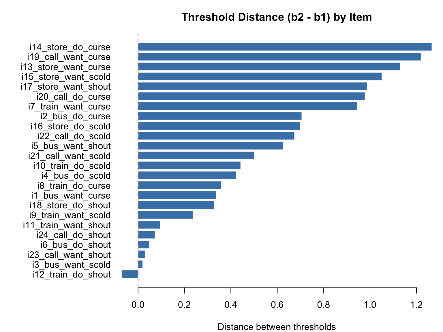

Items with larger threshold distances have a wider region of \(\theta\) where the middle category (“perhaps”) is the most probable response. Items with very small or negative threshold distances may indicate problems with the middle category.

18.4 Category Response Curves

The Category Response Curves (CRCs) show the probability of each response category as a function of \(\theta\).

# Show CRCs for two items: a want/do pair
plot(pcm, type = "trace", which.items = c(7, 8),
     theta_lim = c(-4, 4), par.settings = simpleTheme(lwd = 2),
     main = "PCM Category Response Curves: Item 7 (want) vs. Item 8 (do)")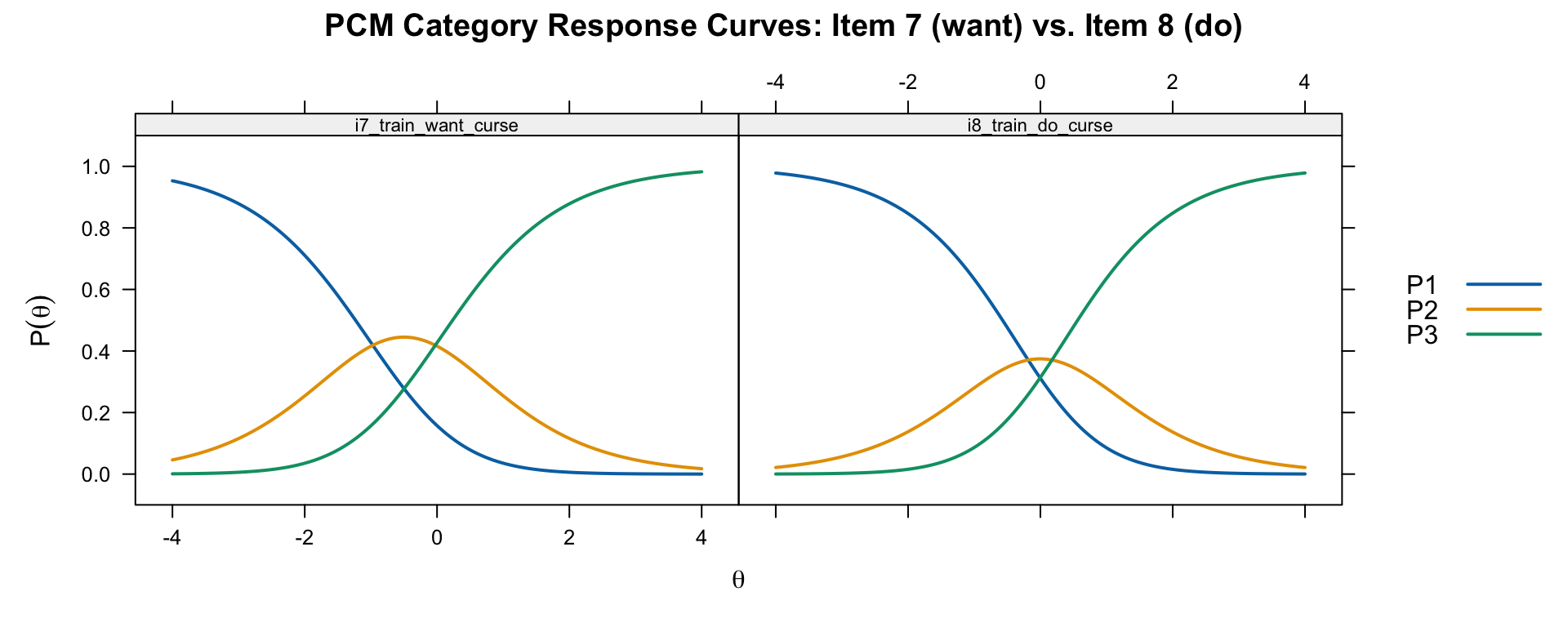

Item 7 is “I miss a train because a clerk gave me faulty information. I would want to curse.” Item 8 is the same situation but “I would curse.” Compare the location and spacing of the thresholds: the “do” item should generally require more verbal aggression (higher \(\theta\)) than the “want” item.

# All 24 items
plot(pcm, type = "trace", theta_lim = c(-4, 4),
     par.settings = simpleTheme(lwd = 2),
     layout = c(4, 6))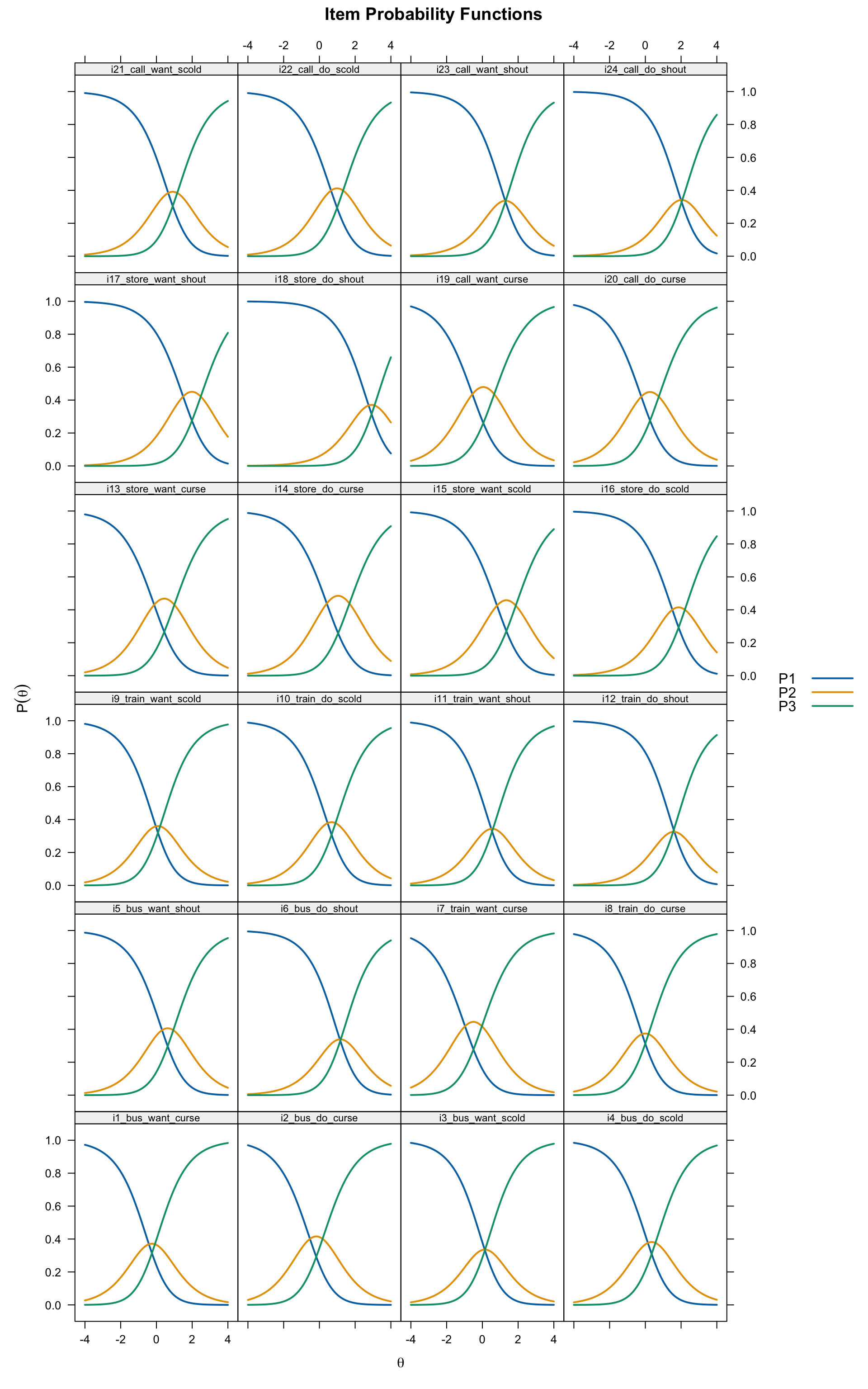

18.5 Threshold Reversals

Sometimes the PCM threshold estimates are disordered (i.e., \(b_2 < b_1\)), meaning the second threshold is easier than the first. When this happens, the middle category is never the most probable response for any value of \(\theta\).

reversed <- which(pcm_pars[, "b2"] < pcm_pars[, "b1"])
if (length(reversed) > 0) {
  cat("Items with reversed thresholds:", paste(reversed, collapse = ", "), "\n")
  cat("These items' middle category ('perhaps') is never the most likely response.\n")
} else {
  cat("No threshold reversals detected.\n")
}

Items with reversed thresholds: 12 
These items' middle category ('perhaps') is never the most likely response.

What do reversals indicate? There are two perspectives:

• Embretson & Reise (2000) take a pragmatic view: reversals simply indicate that a category is never the modal response. They are “not necessarily problematic.”
• Andrich (2015) argues more strongly: “Because the successive categories are intended to be ordered in the sense that they successively reflect more of the trait, the implication is that the thresholds which define the boundaries of the categories are not only expected, but required to increase in difficulty.” Reversed thresholds signal a problem with how the categories are functioning empirically.

It is important to note that Andrich (2015) also clarifies that threshold parameters are not “steps” in a sequential process. A person does not “step through” categories sequentially to arrive at their response. Rather, the thresholds are difficulty parameters that define the boundaries between adjacent categories on the latent trait continuum.

18.6 Wright Map

The Wright map (also called a person-item map) displays the distribution of person abilities alongside item threshold locations on the same scale.

# Custom Wright map: person distribution + item thresholds
theta_est <- fscores(pcm, method = "EAP")[, 1]

layout(matrix(c(1, 2), nrow = 1), widths = c(1, 2))

# Left panel: person distribution
par(mar = c(4, 1, 3, 0))
hist_data <- hist(theta_est, breaks = 30, plot = FALSE)
barplot(hist_data$counts, horiz = TRUE, space = 0, col = "steelblue",
        border = "white", axes = FALSE,
        main = "Persons")
axis(1)

# Right panel: item thresholds
par(mar = c(4, 4, 3, 1))
plot(NA, xlim = c(-4, 4), ylim = c(0.5, 24.5),
     xlab = expression(theta), ylab = "", yaxt = "n",
     main = "Item Thresholds (PCM)")
axis(2, at = 1:24, labels = 1:24, las = 1, cex.axis = 0.7)
abline(h = 1:24, col = "grey90")

for (i in 1:24) {
  points(pcm_pars[i, "b1"], i, pch = 1, col = "red", cex = 1.2)
  points(pcm_pars[i, "b2"], i, pch = 2, col = "blue", cex = 1.2)
}
legend("topright", legend = c("b1 (0|1)", "b2 (1|2)"),
       pch = c(1, 2), col = c("red", "blue"), bty = "n")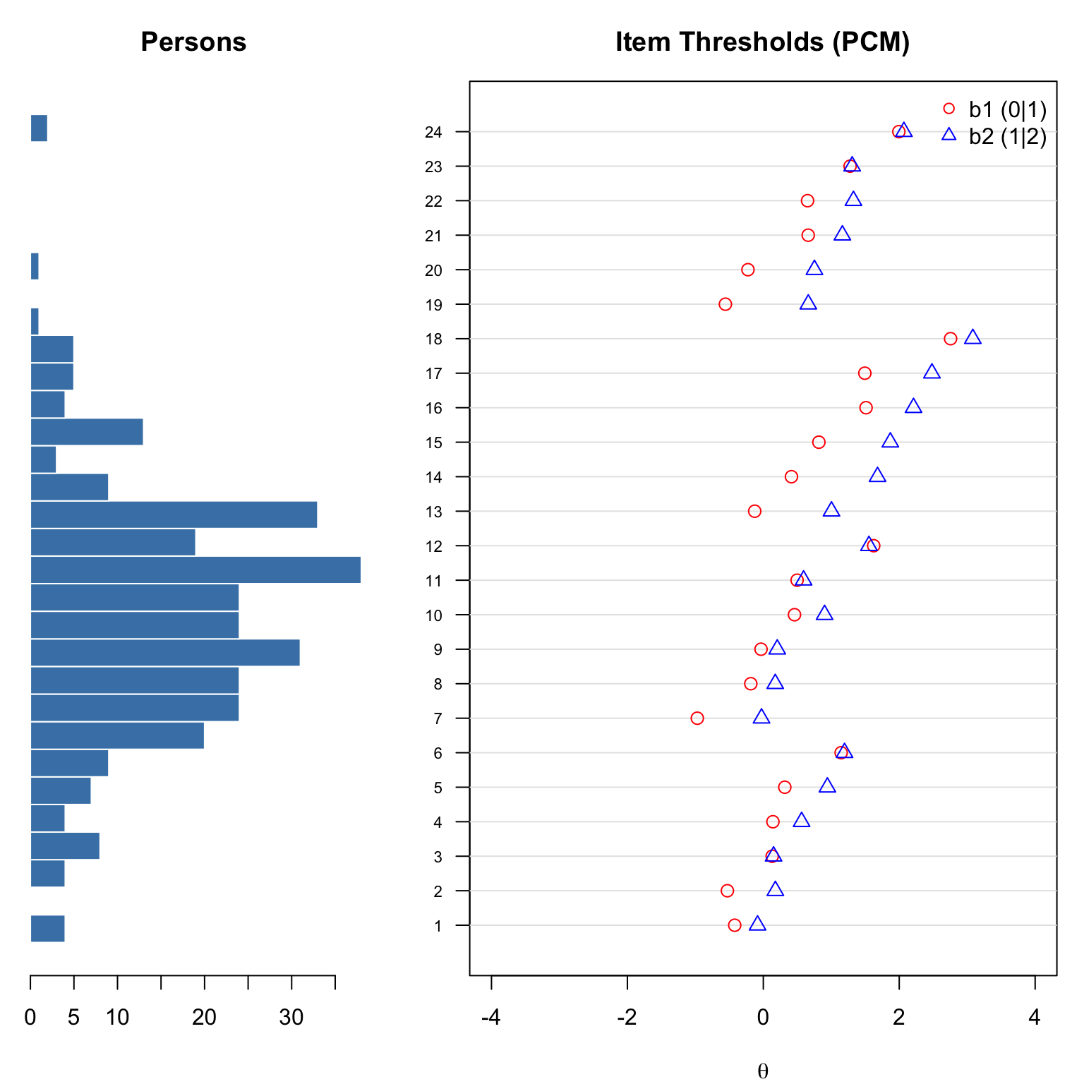

layout(1)

18.7 Comparing Want vs. Do Items

One of our motivating questions concerns the difference between “want to” and “do” items. Let’s compare threshold estimates for matched want/do pairs.

# Compare CRCs for want vs. do pairs
# Items 1&2 (bus, curse), 7&8 (train, curse), 9&10 (train, scold), 23&24 (call, shout)
plot(pcm, type = "trace",
     which.items = c(1, 2, 7, 8, 9, 10, 23, 24),
     theta_lim = c(-4, 4),
     par.settings = simpleTheme(lwd = 2),
     layout = c(2, 4))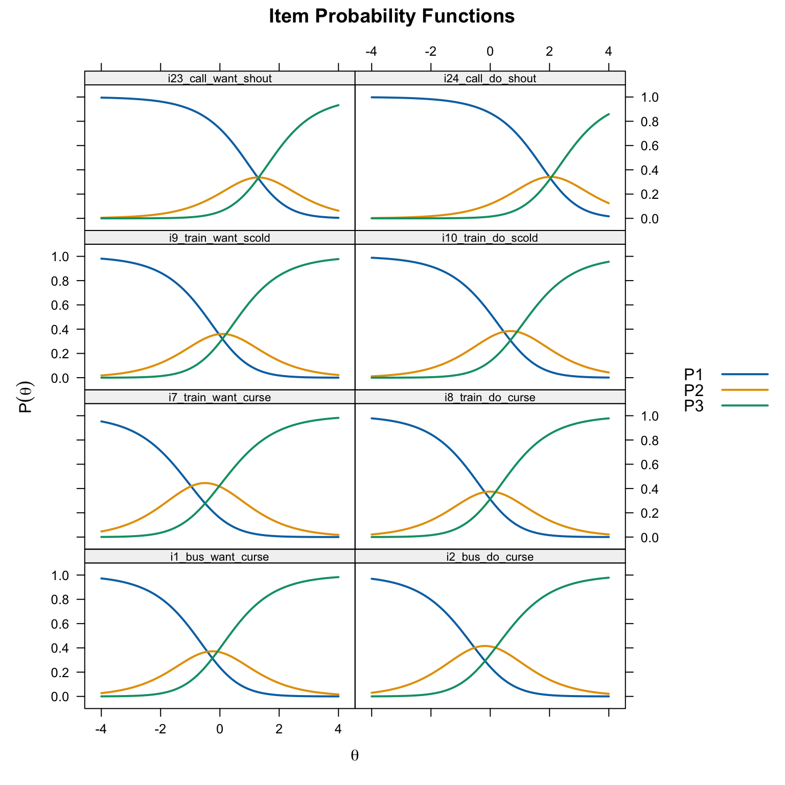

Within each pair, the “do” item (even-numbered) should generally have thresholds located further to the right (higher \(\theta\)) than the “want” item (odd-numbered), reflecting the greater verbal aggression needed to endorse actually doing the behavior vs. merely wanting to.

19 Generalized Partial Credit Model (GPCM)

19.1 Model Overview

The Generalized Partial Credit Model (Muraki, 1992) extends the PCM by allowing each item to have its own discrimination parameter (\(a_i\)):

\[P(X_{ij} = k \mid \theta_j) = \frac{\exp\left(\sum_{v=0}^{k} a_i(\theta_j - b_{iv})\right)}{\sum_{r=0}^{m}\exp\left(\sum_{v=0}^{r} a_i(\theta_j - b_{iv})\right)}\]

The GPCM is to the PCM as the 2PL is to the Rasch model for dichotomous items. When all \(a_i = 1\), the GPCM reduces to the PCM.

A note on sufficiency: Andrich (2015) points out that adding item-specific discrimination parameters “destroys sufficiency”—the total score is no longer a sufficient statistic for \(\theta\). From a measurement perspective (as opposed to a statistical modeling perspective), this is a significant trade-off.

19.2 Fitting the GPCM

gpcm <- mirt(d, 1, itemtype = "gpcm")

19.3 Parameter Estimates

gpcm_pars <- coef(gpcm, IRTpars = TRUE, simplify = TRUE)$items
colnames(gpcm_pars) <- c("a", "b1", "b2")
knitr::kable(round(gpcm_pars, 3),
             caption = "GPCM Parameter Estimates")

GPCM Parameter Estimates

	a	b1	b2
i1_bus_want_curse	0.782	-0.402	-0.184
i2_bus_do_curse	1.184	-0.542	0.229
i3_bus_want_scold	1.011	0.120	0.175
i4_bus_do_scold	1.565	-0.006	0.609
i5_bus_want_shout	0.831	0.415	1.012
i6_bus_do_shout	0.917	1.251	1.241
i7_train_want_curse	0.871	-1.036	-0.054
i8_train_do_curse	1.158	-0.227	0.233
i9_train_want_scold	0.919	-0.010	0.201
i10_train_do_scold	1.536	0.262	0.886
i11_train_want_shout	0.873	0.596	0.603
i12_train_do_shout	1.169	1.436	1.542
i13_store_want_curse	0.645	-0.055	1.235
i14_store_do_curse	0.883	0.479	1.809
i15_store_want_scold	1.018	0.812	1.884
i16_store_do_scold	1.228	1.296	2.094
i17_store_want_shout	0.865	1.696	2.685
i18_store_do_shout	0.974	2.830	3.164
i19_call_want_curse	0.740	-0.614	0.745
i20_call_do_curse	0.925	-0.223	0.788
i21_call_want_scold	1.111	0.595	1.161
i22_call_do_scold	1.207	0.542	1.284
i23_call_want_shout	0.686	1.824	1.470
i24_call_do_shout	0.899	2.193	2.172

Now each item has its own discrimination (\(a\)) parameter in addition to two thresholds. Items with higher \(a\) values discriminate more sharply between trait levels near the thresholds.

# Plot discrimination parameters
par(mar = c(4, 11, 3, 1))
barplot(sort(gpcm_pars[, "a"]), horiz = TRUE,
        names.arg = rownames(gpcm_pars)[order(gpcm_pars[, "a"])],
        las = 1, col = "steelblue", border = "white",
        main = "GPCM Item Discrimination Parameters",
        xlab = "Discrimination (a)")
abline(v = 1, col = "red", lty = 2)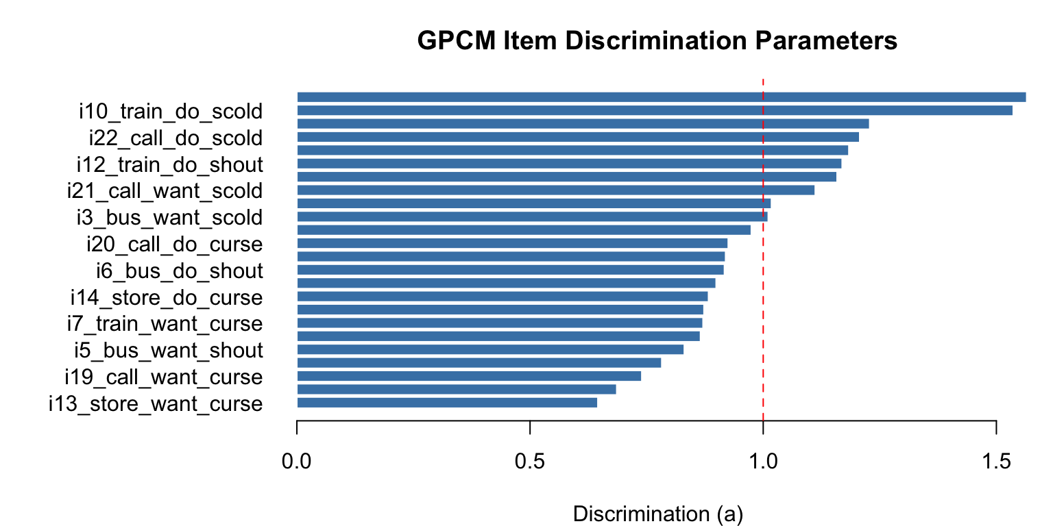

The dashed line at \(a = 1\) represents the PCM constraint. Items above this line discriminate more than assumed by the PCM; items below discriminate less.

19.4 Category Response Curves

# Compare same want/do pairs under GPCM
plot(gpcm, type = "trace",
     which.items = c(1, 2, 7, 8, 9, 10, 23, 24),
     theta_lim = c(-4, 4),
     par.settings = simpleTheme(lwd = 2),
     layout = c(2, 4))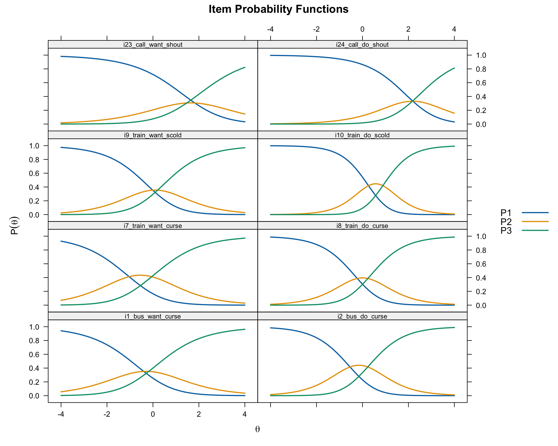

Compare these CRCs to the PCM versions above. Items with high discrimination will have narrower, more peaked curves; items with low discrimination will have flatter, wider curves.

# Check for reversals
gpcm_reversed <- which(gpcm_pars[, "b2"] < gpcm_pars[, "b1"])
if (length(gpcm_reversed) > 0) {
  cat("Items with reversed thresholds under GPCM:",
      paste(gpcm_reversed, collapse = ", "), "\n")
} else {
  cat("No threshold reversals under GPCM.\n")
}

Items with reversed thresholds under GPCM: 6, 23, 24 

One reason to fit the GPCM when the PCM shows reversals is that the reversals may be an artifact of assuming equal discrimination. If items actually vary in their discrimination, the PCM misattributes this variation, which can distort threshold estimates.

20 Rating Scale Model (RSM)

20.1 Model Overview

The Rating Scale Model (Andrich, 1978) is a special case of the PCM in which the threshold distances are constrained to be the same across all items. Each item has a single location parameter (\(\lambda_i\)), and the category structure is defined by a common set of threshold parameters (\(\tau_k\)) shared by all items:

\[P(X_{ij} = k \mid \theta_j) = \frac{\exp\left(\sum_{v=0}^{k}(\theta_j - \lambda_i - \tau_v)\right)}{\sum_{r=0}^{m}\exp\left(\sum_{v=0}^{r}(\theta_j - \lambda_i - \tau_v)\right)}\]

The RSM is appropriate when all items share the same response format and the distances between categories can reasonably be assumed equal across items. This is a strong assumption—whether it holds is an empirical question.

Key implication: Under the RSM, the CRCs for all items have the same shape; they are simply shifted left or right along the \(\theta\) axis according to each item’s location parameter.

20.1.1 From Log-Odds to Category Probabilities

The RSM is often stated in its log-odds form:

\[\ln\frac{P(X_{ij} = k)}{P(X_{ij} = k-1)} = \theta_j - \lambda_i - \tau_k\]

The category probability equations follow directly from this. Here is the step-by-step derivation for a three-category item (categories 0, 1, 2):

Step 1. Exponentiate both sides for each adjacent pair:

\[\frac{P(X=1)}{P(X=0)} = \exp(\theta_j - \lambda_i - \tau_1), \qquad \frac{P(X=2)}{P(X=1)} = \exp(\theta_j - \lambda_i - \tau_2)\]

Step 2. Rearrange to express higher categories in terms of the one below:

\[P(X=1) = P(X=0) \cdot \exp(\theta_j - \lambda_i - \tau_1)\] \[P(X=2) = P(X=1) \cdot \exp(\theta_j - \lambda_i - \tau_2)\]

Step 3. Substitute the expression for \(P(X=1)\) into \(P(X=2)\):

\[P(X=2) = P(X=0) \cdot \exp(\theta_j - \lambda_i - \tau_1) \cdot \exp(\theta_j - \lambda_i - \tau_2) = P(X=0) \cdot \exp(2\theta_j - 2\lambda_i - \tau_1 - \tau_2)\]

Step 4. Use the requirement that all probabilities sum to 1:

\[P(X=0)\left[1 + \exp(\theta_j - \lambda_i - \tau_1) + \exp(2\theta_j - 2\lambda_i - \tau_1 - \tau_2)\right] = 1\]

Defining \(\Psi\) as the bracketed denominator, we get \(P(X=0) = 1/\Psi\), \(P(X=1) = \exp(\theta_j - \lambda_i - \tau_1)/\Psi\), and \(P(X=2) = \exp(2\theta_j - 2\lambda_i - \tau_1 - \tau_2)/\Psi\).

The key insight from Step 3 is that each additional category requires multiplying in one more log-odds term. This is why the exponent for category \(k\) contains \(k\) copies of \(\theta_j\) and \(\lambda_i\), and accumulates all \(\tau\) parameters up through \(\tau_k\).

20.2 Fitting the RSM

rsm <- mirt(d, 1, itemtype = "rsm")

20.3 Parameter Estimates

rsm_pars <- as.data.frame(coef(rsm, simplify = TRUE)$items)

In mirt’s RSM output (without IRTpars = TRUE), the columns are:

• b1 = \(\tau_1\): the first common Andrich threshold (same for all items)
• b2 = \(\tau_2\): the second common Andrich threshold (same for all items)
• c = \(-\lambda_i\): the item-specific location parameter (varies by item)

To recover the adjacent category intersection thresholds (\(t_k = \lambda_i + \tau_k\)) for each item, we use \(t_k = -c_i + b_k\):

rsm_thresh <- data.frame(
  t1 = -rsm_pars[, "c"] + rsm_pars[, "b1"],
  t2 = -rsm_pars[, "c"] + rsm_pars[, "b2"]
)
knitr::kable(round(rsm_thresh, 3),
             caption = "RSM Andrich Threshold Estimates")

RSM Andrich Threshold Estimates

t1	t2
-0.552	0.028
-0.464	0.116
-0.143	0.438
0.067	0.648
0.334	0.915
0.952	1.532
-0.766	-0.185
-0.297	0.284
-0.203	0.378
0.400	0.980
0.284	0.864
1.418	1.999
0.115	0.696
0.661	1.242
0.970	1.551
1.543	2.123
1.595	2.176
2.712	3.293
-0.243	0.337
-0.042	0.539
0.629	1.210
0.685	1.266
1.084	1.665
1.861	2.442

Under the RSM, the distance between thresholds (\(t_2 - t_1 = \tau_2 - \tau_1\)) is the same for all items—only the overall item location \(\lambda_i\) shifts them left or right. Compare the t2 - t1 column: it should be constant across all 24 items (within rounding).

# Item locations: λᵢ = -cᵢ (midpoint of the two thresholds when τ₁ + τ₂ = 0)
rsm_locations <- -rsm_pars[, "c"]

20.4 Category Response Curves

# Compare same want/do pair under RSM
plot(rsm, type = "trace", which.items = c(7, 8),
     theta_lim = c(-4, 4), par.settings = simpleTheme(lwd = 2),
     main = "RSM Category Response Curves: Item 7 vs. Item 8")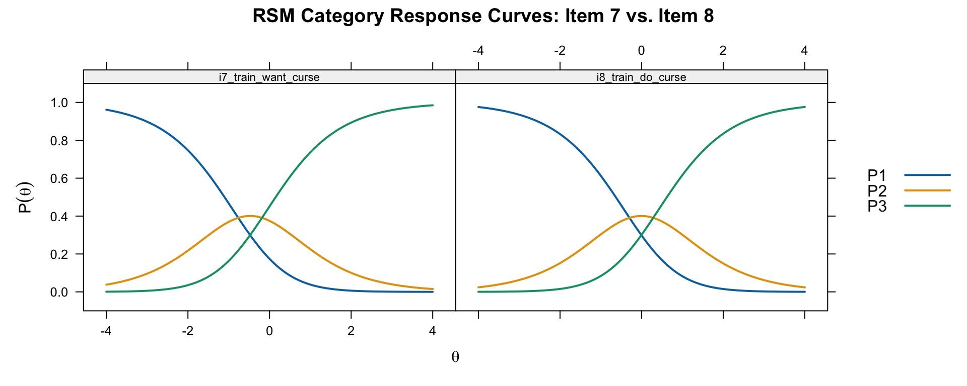

Notice that the CRCs have the same shape for both items—they differ only in their horizontal location. This is the defining property of the RSM.

20.5 Wright Map

# Custom Wright map for RSM
theta_est_rsm <- fscores(rsm, method = "EAP")[, 1]

# rsm_thresh (t1, t2) already computed correctly above

layout(matrix(c(1, 2), nrow = 1), widths = c(1, 2))

# Left panel: person distribution
par(mar = c(4, 1, 3, 0))
hist_data <- hist(theta_est_rsm, breaks = 30, plot = FALSE)
barplot(hist_data$counts, horiz = TRUE, space = 0, col = "steelblue",
        border = "white", axes = FALSE,
        main = "Persons")
axis(1)

# Right panel: item thresholds
par(mar = c(4, 4, 3, 1))
plot(NA, xlim = c(-4, 4), ylim = c(0.5, 24.5),
     xlab = expression(theta), ylab = "", yaxt = "n",
     main = "Item Thresholds (RSM)")
axis(2, at = 1:24, labels = 1:24, las = 1, cex.axis = 0.7)
abline(h = 1:24, col = "grey90")

for (i in 1:24) {
  points(rsm_thresh[i, "t1"], i, pch = 1, col = "red", cex = 1.2)
  points(rsm_thresh[i, "t2"], i, pch = 2, col = "blue", cex = 1.2)
}
legend("topright", legend = c("t1 (0|1)", "t2 (1|2)"),
       pch = c(1, 2), col = c("red", "blue"), bty = "n")

layout(1)

Compare this to the PCM Wright map. Under the RSM, the distance between each item’s thresholds is constant, so the map has a more regular appearance.

20.6 PCM vs. RSM: Which Fits Better?

anova(rsm, pcm)

         AIC    SABIC       HQ      BIC    logLik     X2 df p
rsm 12743.68 12758.86 12782.69 12841.33 -6345.840            
pcm 12737.47 12766.08 12810.99 12921.50 -6319.733 52.214 23 0

This likelihood ratio test compares the constrained RSM (equal threshold distances) to the more flexible PCM (item-specific threshold distances). A significant result suggests the PCM provides a meaningfully better fit, and the RSM’s constraint is too restrictive for these data.

21 Graded Response Model (GRM)

21.1 Model Overview

The Graded Response Model (Samejima, 1969) takes a fundamentally different approach from the adjacent-category models above. Rather than modeling the probability of one category vs. an adjacent category, the GRM models the cumulative probability of responding at or above each category threshold.

For each item, the GRM first estimates \(m\) operating characteristic curves (OCCs):

\[P^*_{ik}(\theta) = \frac{\exp[a_i(\theta - b_{ik})]}{1 + \exp[a_i(\theta - b_{ik})]}\]

where \(b_{ik}\) is the Thurstonian threshold—the \(\theta\) value where there is a 50% chance of responding at or above category \(k\). These OCCs are simply 2PL curves.

The probability of responding in a specific category is then obtained by subtraction:

\[P(X_{ij} = k \mid \theta_j) = P^*_{ik}(\theta) - P^*_{i,k+1}(\theta)\]

with the boundary conditions \(P^*_{i0}(\theta) = 1\) and \(P^*_{i,m+1}(\theta) = 0\).

Key distinction: The GRM thresholds (\(b_{ik}\)) are “Thurstonian” thresholds—they represent the \(\theta\) where the cumulative probability equals 0.50. These are not the same as the “Andrich” thresholds in the PCM/RSM, which represent the \(\theta\) where two adjacent categories are equally likely. This is an important conceptual difference that can lead to confusion when comparing across models.

Important property: In the GRM, the thresholds are always ordered (\(b_{i1} < b_{i2} < \ldots < b_{im}\)) by mathematical necessity. This contrasts with the PCM, where threshold reversals are possible and diagnostically meaningful.

21.2 Fitting the GRM

grm <- mirt(d, 1, itemtype = "graded")

21.3 Parameter Estimates

grm_pars <- coef(grm, IRTpars = TRUE, simplify = TRUE)$items
colnames(grm_pars) <- c("a", "b1", "b2")
knitr::kable(round(grm_pars, 3),
             caption = "GRM Parameter Estimates (Thurstonian Thresholds)")

GRM Parameter Estimates (Thurstonian Thresholds)

	a	b1	b2
i1_bus_want_curse	1.201	-0.947	0.380
i2_bus_do_curse	1.526	-0.807	0.495
i3_bus_want_scold	1.484	-0.391	0.647
i4_bus_do_scold	2.015	-0.201	0.825
i5_bus_want_shout	1.137	-0.045	1.515
i6_bus_do_shout	1.340	0.660	1.860
i7_train_want_curse	1.164	-1.393	0.296
i8_train_do_curse	1.528	-0.566	0.585
i9_train_want_scold	1.314	-0.499	0.709
i10_train_do_scold	1.906	0.052	1.128
i11_train_want_shout	1.242	-0.012	1.192
i12_train_do_shout	1.518	1.010	2.141
i13_store_want_curse	0.913	-0.485	1.638
i14_store_do_curse	1.143	0.192	2.141
i15_store_want_scold	1.301	0.521	2.243
i16_store_do_scold	1.493	1.021	2.536
i17_store_want_shout	1.017	1.314	3.515
i18_store_do_shout	1.090	2.461	4.550
i19_call_want_curse	0.976	-0.971	1.103
i20_call_do_curse	1.251	-0.494	1.104
i21_call_want_scold	1.478	0.259	1.533
i22_call_do_scold	1.541	0.265	1.592
i23_call_want_shout	0.945	0.965	2.536
i24_call_do_shout	1.179	1.569	3.097

21.4 Operating Characteristic Curves

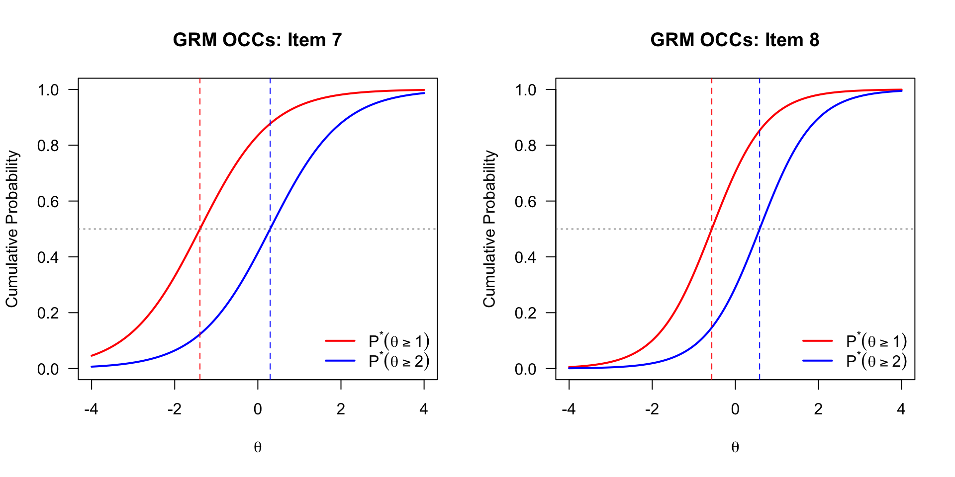
The OCCs show the cumulative probability of responding at or above each threshold.

# Custom OCCs (cumulative probability curves) for Items 7 and 8
theta_seq <- seq(-4, 4, length.out = 200)

par(mfrow = c(1, 2))

for (item in c(7, 8)) {
  a <- grm_pars[item, "a"]
  b1 <- grm_pars[item, "b1"]
  b2 <- grm_pars[item, "b2"]

  # P*(theta) = probability of responding at or above category k
  p_star1 <- 1 / (1 + exp(-a * (theta_seq - b1)))
  p_star2 <- 1 / (1 + exp(-a * (theta_seq - b2)))

  plot(theta_seq, p_star1, type = "l", col = "red", lwd = 2,
       xlab = expression(theta), ylab = "Cumulative Probability",
       main = paste("GRM OCCs: Item", item),
       ylim = c(0, 1), las = 1)
  lines(theta_seq, p_star2, col = "blue", lwd = 2)
  abline(h = 0.5, lty = 3, col = "grey50")
  abline(v = c(b1, b2), lty = 2, col = c("red", "blue"))
  legend("bottomright",
         legend = c(expression(P^"*"*(theta >= 1)),
                    expression(P^"*"*(theta >= 2))),
         col = c("red", "blue"), lwd = 2, bty = "n")
}

par(mfrow = c(1, 1))

21.5 Category Response Curves

# CRCs
plot(grm, type = "trace", which.items = c(7, 8),
     theta_lim = c(-4, 4), par.settings = simpleTheme(lwd = 2),
     main = "GRM Category Response Curves: Item 7 vs. Item 8")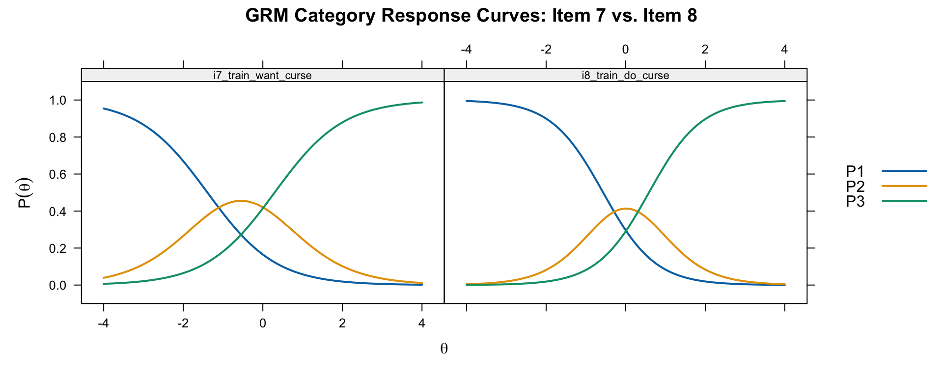

Compare these GRM category response curves to the PCM curves for the same items. Two sources of difference are worth noting. First, because the GRM estimates an item-specific discrimination parameter (\(a_i\)), items with high discrimination will have narrower, more peaked curves than the PCM’s equal-discrimination curves. Second, even holding discrimination constant, the GRM and PCM use fundamentally different mathematical forms—the GRM derives category probabilities by subtracting adjacent cumulative logistic curves, while the PCM uses adjacent-category ratios—and these different forms can produce different CRC shapes and peak locations. Note that the Thurstonian vs. Andrich threshold distinction explains why the numerical parameter values are not directly comparable across the two models, but is not itself the reason the CRCs look different: the curves reflect the fitted probabilities directly, regardless of how the underlying threshold parameters are defined.

# All 24 items
plot(grm, type = "trace", theta_lim = c(-4, 4),
     par.settings = simpleTheme(lwd = 2),
     layout = c(4, 6))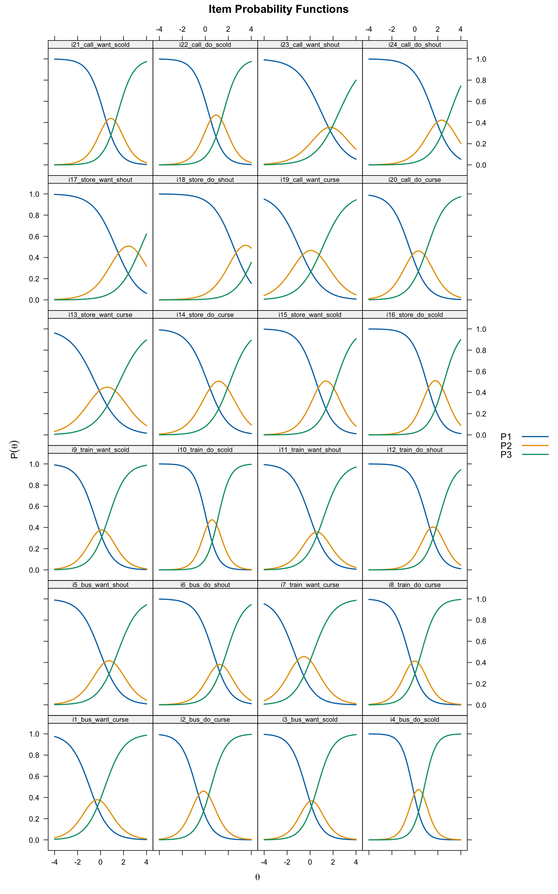

21.6 Item and Test Information

One advantage of the GRM (and other models with item-specific discrimination) is the ability to examine differential item information.

# Test information
plot(grm, type = "info", theta_lim = c(-4, 4))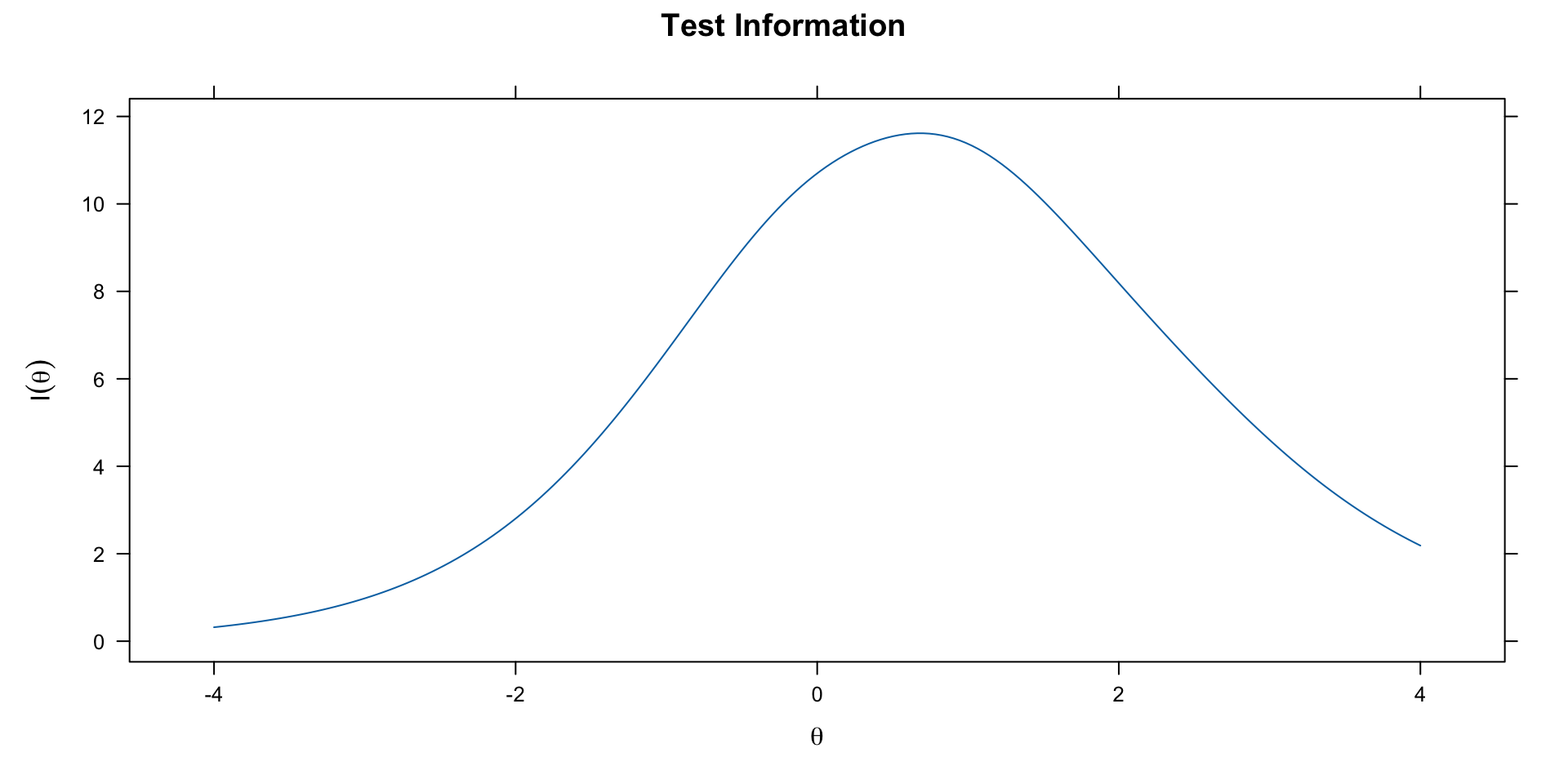

The test information function tells us where on the \(\theta\) scale the test provides the most precise measurement. Items with higher discrimination contribute more information, particularly near their threshold locations.

22 Model Comparison

22.1 Comparing Model Fit

We can compare nested and non-nested models using information criteria (AIC, BIC) and likelihood ratio tests where appropriate.

# Extract fit indices using anova() on individual models
fit_rsm  <- anova(rsm)
fit_pcm  <- anova(pcm)
fit_gpcm <- anova(gpcm)
fit_grm  <- anova(grm)

fits <- data.frame(
  Model  = c("RSM", "PCM", "GPCM", "GRM"),
  AIC    = c(fit_rsm$AIC,  fit_pcm$AIC,  fit_gpcm$AIC,  fit_grm$AIC),
  BIC    = c(fit_rsm$BIC,  fit_pcm$BIC,  fit_gpcm$BIC,  fit_grm$BIC),
  logLik = c(fit_rsm$logLik, fit_pcm$logLik, fit_gpcm$logLik, fit_grm$logLik)
)
knitr::kable(fits, digits = 1, caption = "Model Fit Comparison (lower AIC/BIC = better)")

Model Fit Comparison (lower AIC/BIC = better)

Model	AIC	BIC	logLik
RSM	12743.7	12841.3	-6345.8
PCM	12737.5	12921.5	-6319.7
GPCM	12741.0	13011.4	-6298.5
GRM	12715.6	12986.0	-6285.8

Nested comparisons:

• RSM is nested within PCM (test whether threshold distances are equal across items):

anova(rsm, pcm)

         AIC    SABIC       HQ      BIC    logLik     X2 df p
rsm 12743.68 12758.86 12782.69 12841.33 -6345.840            
pcm 12737.47 12766.08 12810.99 12921.50 -6319.733 52.214 23 0

• PCM is nested within GPCM (test whether discrimination is equal across items):

anova(pcm, gpcm)

          AIC    SABIC       HQ      BIC    logLik     X2 df     p
pcm  12737.47 12766.08 12810.99 12921.50 -6319.733                
gpcm 12740.99 12783.04 12849.02 13011.41 -6298.497 42.474 23 0.008

Note that the GRM is not nested within the PCM/GPCM family—they are based on different response process assumptions. We can still compare them via AIC/BIC.

22.2 Comparing Parameter Estimates Across Models

par(mfrow = c(1, 2))

# Compare b1 across models
plot(pcm_pars[, "b1"], gpcm_pars[, "b1"],
     xlab = "PCM b1", ylab = "GPCM b1",
     main = "Threshold 1: PCM vs. GPCM", pch = 16, col = "steelblue")
abline(0, 1, lty = 2, col = "red")
text(pcm_pars[, "b1"], gpcm_pars[, "b1"], labels = 1:24, pos = 3, cex = 0.7)
r1 <- cor(pcm_pars[, "b1"], gpcm_pars[, "b1"])
legend("topleft", legend = paste("r =", round(r1, 3)), bty = "n")

# Compare b2 across models
plot(pcm_pars[, "b2"], gpcm_pars[, "b2"],
     xlab = "PCM b2", ylab = "GPCM b2",
     main = "Threshold 2: PCM vs. GPCM", pch = 16, col = "steelblue")
abline(0, 1, lty = 2, col = "red")
text(pcm_pars[, "b2"], gpcm_pars[, "b2"], labels = 1:24, pos = 3, cex = 0.7)
r2 <- cor(pcm_pars[, "b2"], gpcm_pars[, "b2"])
legend("topleft", legend = paste("r =", round(r2, 3)), bty = "n")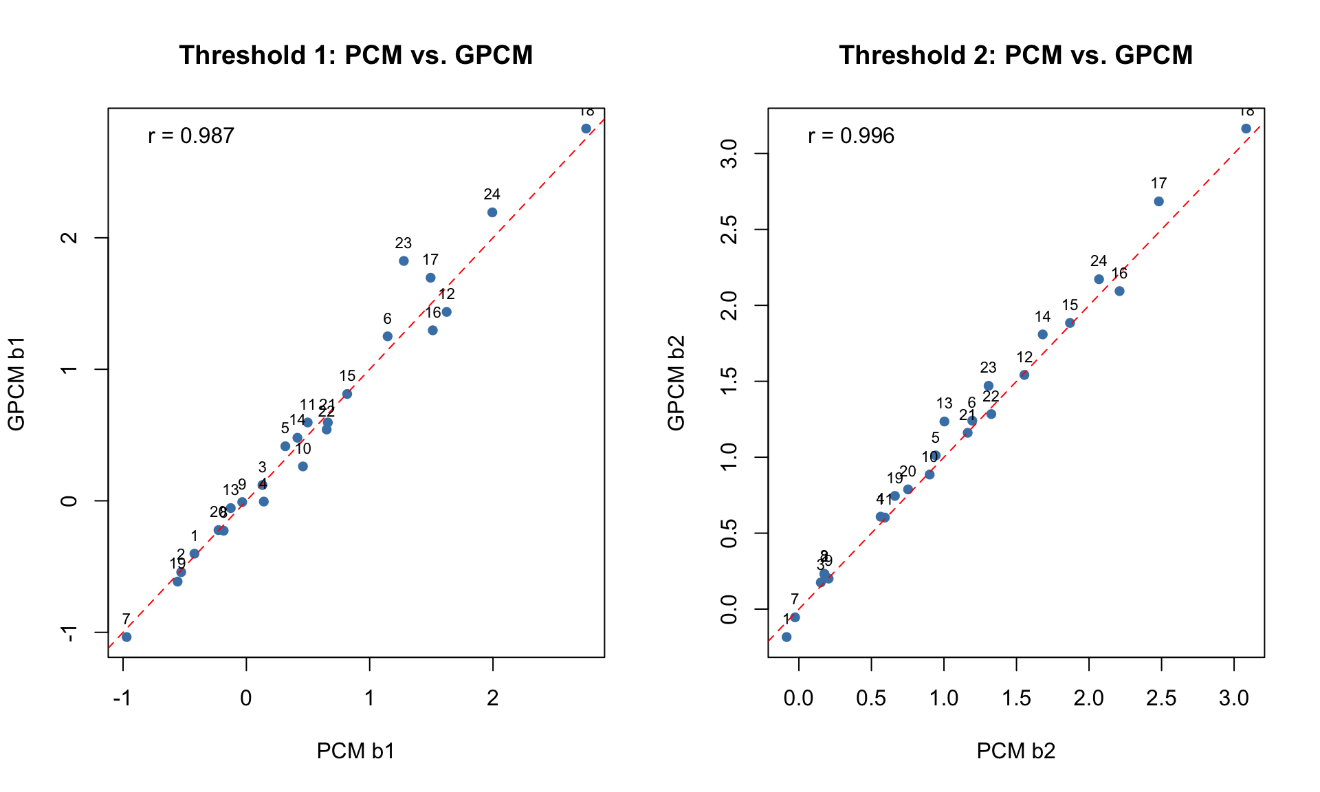

par(mfrow = c(1, 1))

par(mfrow = c(1, 2))

# Compare GPCM vs GRM thresholds
plot(gpcm_pars[, "b1"], grm_pars[, "b1"],
     xlab = "GPCM b1", ylab = "GRM b1",
     main = "Threshold 1: GPCM vs. GRM", pch = 16, col = "darkorange")
abline(0, 1, lty = 2, col = "red")
text(gpcm_pars[, "b1"], grm_pars[, "b1"], labels = 1:24, pos = 3, cex = 0.7)

plot(gpcm_pars[, "b2"], grm_pars[, "b2"],
     xlab = "GPCM b2", ylab = "GRM b2",
     main = "Threshold 2: GPCM vs. GRM", pch = 16, col = "darkorange")
abline(0, 1, lty = 2, col = "red")
text(gpcm_pars[, "b2"], grm_pars[, "b2"], labels = 1:24, pos = 3, cex = 0.7)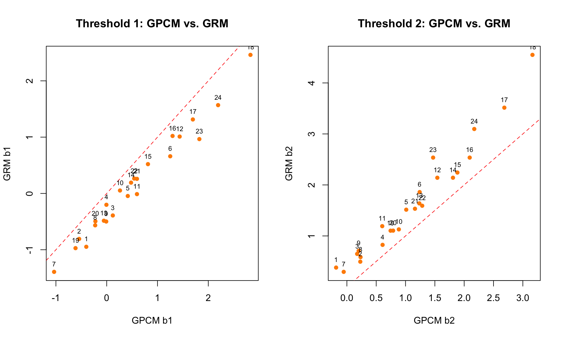

par(mfrow = c(1, 1))

Notice that the GPCM and GRM thresholds may not align closely on the identity line. This is expected because they represent different quantities: Andrich thresholds (adjacent category crossover) vs. Thurstonian thresholds (cumulative 50% point).

22.3 Returning to the Motivating Questions

# Q1: Which items require the most verbal aggression?
# Use GRM b2 (threshold for "yes") as the benchmark
cat("Items requiring the MOST verbal aggression (highest b2, GRM):\n")

Items requiring the MOST verbal aggression (highest b2, GRM):

top5 <- head(order(grm_pars[, "b2"], decreasing = TRUE), 5)
for (i in top5) {
  cat(sprintf("  Item %d (%s): b2 = %.2f\n", i, names(d)[i], grm_pars[i, "b2"]))
}

  Item 18 (i18_store_do_shout): b2 = 4.55
  Item 17 (i17_store_want_shout): b2 = 3.51
  Item 24 (i24_call_do_shout): b2 = 3.10
  Item 16 (i16_store_do_scold): b2 = 2.54
  Item 23 (i23_call_want_shout): b2 = 2.54

cat("\nItems requiring the LEAST verbal aggression (lowest b2, GRM):\n")

Items requiring the LEAST verbal aggression (lowest b2, GRM):

bot5 <- head(order(grm_pars[, "b2"]), 5)
for (i in bot5) {
  cat(sprintf("  Item %d (%s): b2 = %.2f\n", i, names(d)[i], grm_pars[i, "b2"]))
}

  Item 7 (i7_train_want_curse): b2 = 0.30
  Item 1 (i1_bus_want_curse): b2 = 0.38
  Item 2 (i2_bus_do_curse): b2 = 0.50
  Item 8 (i8_train_do_curse): b2 = 0.58
  Item 3 (i3_bus_want_scold): b2 = 0.65

# Q2: Threshold distances for want vs. do items
pcm_dist <- pcm_pars[, "b2"] - pcm_pars[, "b1"]
want_items <- seq(1, 23, 2)  # odd items
do_items <- seq(2, 24, 2)    # even items

boxplot(pcm_dist[want_items], pcm_dist[do_items],
        names = c("Want", "Do"), col = c("lightblue", "salmon"),
        main = "PCM Threshold Distances: Want vs. Do Items",
        ylab = "b2 - b1")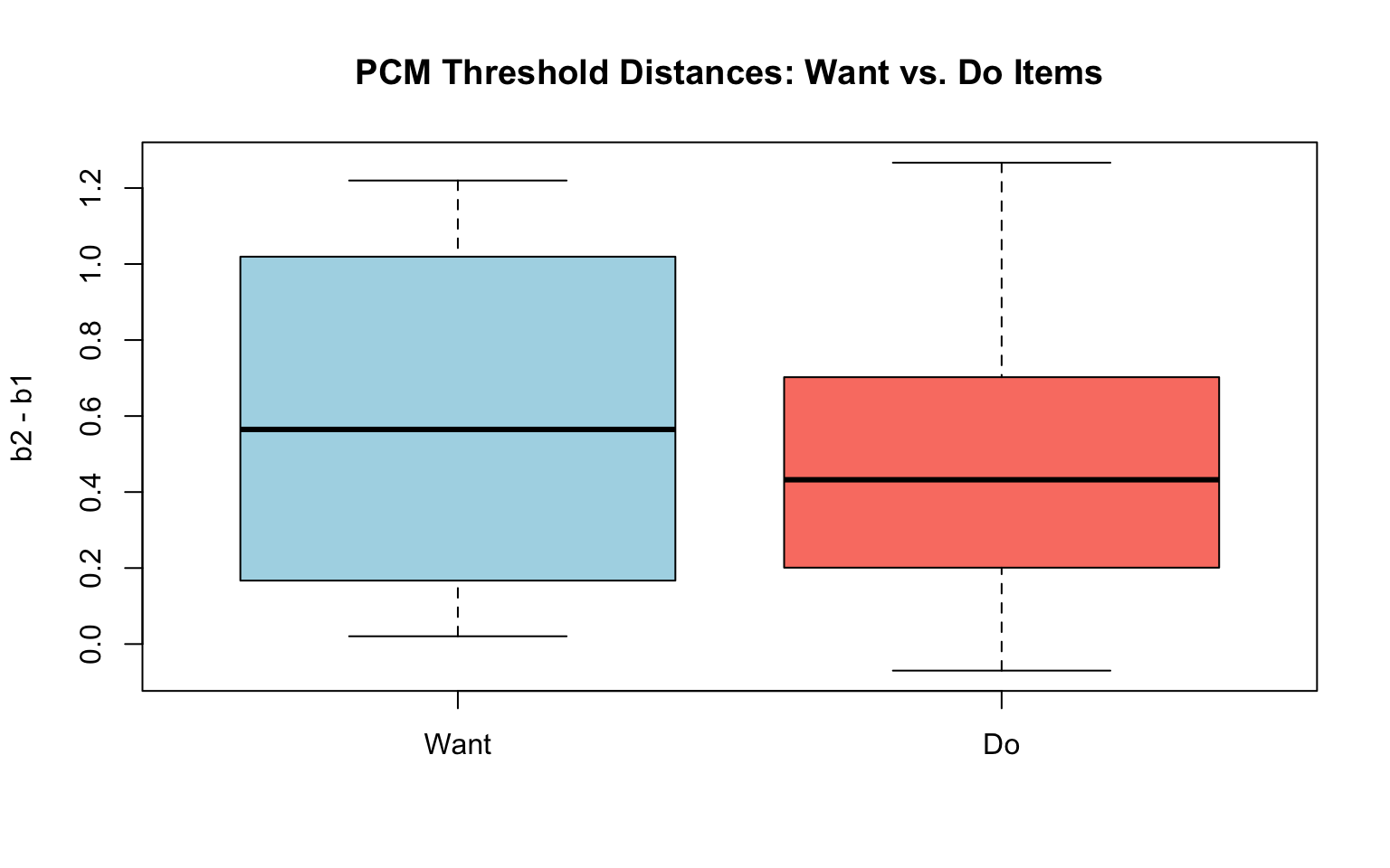

cat("Mean threshold distance (Want):", round(mean(pcm_dist[want_items]), 3), "\n")

Mean threshold distance (Want): 0.599 

cat("Mean threshold distance (Do):", round(mean(pcm_dist[do_items]), 3), "\n")

Mean threshold distance (Do): 0.494 

# Q3: Other-to-blame vs. self-to-blame
other_items <- c(1:12)   # bus and train
self_items <- c(13:24)    # store and call

# Average item location across models
pcm_locs <- rowMeans(pcm_pars[, 2:3])

boxplot(pcm_locs[other_items], pcm_locs[self_items],
        names = c("Other to blame\n(bus, train)", "Self to blame\n(store, call)"),
        col = c("lightblue", "salmon"),
        main = "PCM Item Locations: Blame Attribution",
        ylab = "Average threshold location")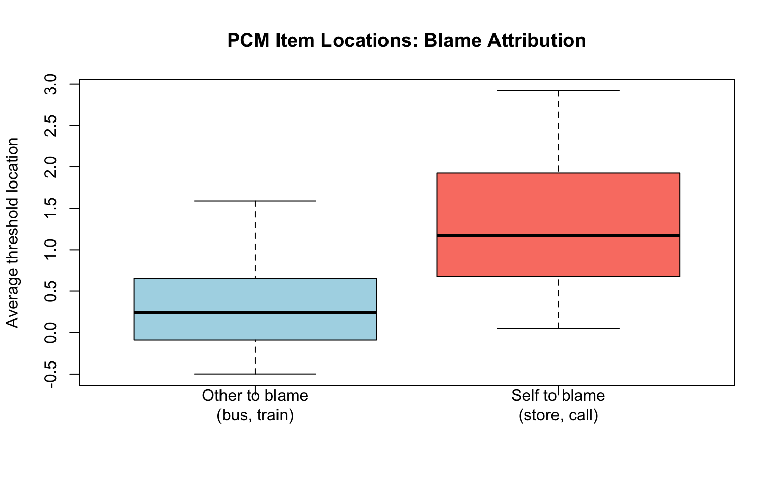

cat("Mean location (Other to blame):", round(mean(pcm_locs[other_items]), 3), "\n")

Mean location (Other to blame): 0.355 

cat("Mean location (Self to blame):", round(mean(pcm_locs[self_items]), 3), "\n")

Mean location (Self to blame): 1.261 

23 Nominal Response Model (NRM)

23.1 Model Overview

The Nominal Response Model (Bock, 1972) does not assume any ordering of the response categories. Instead, it estimates separate slope (\(a_k\)) and intercept (\(c_k\)) parameters for each category:

\[P(X_{ij} = k \mid \theta_j) = \frac{\exp(a_{ik}\theta_j + c_{ik})}{\sum_{r=0}^{m}\exp(a_{ir}\theta_j + c_{ir})}\]

The NRM is the most general model: all other polytomous models can be expressed as special cases with constraints on the \(a_k\) and \(c_k\) parameters.

When is the NRM useful?

• When you want to empirically verify that response categories are ordered as intended.
• For items where categories are truly nominal (e.g., analyzing distractor choice patterns on multiple-choice items).

The mirt package uses a reparameterized version of the NRM that separates an overall item discrimination from empirically derived category weights.

23.2 Fitting the NRM

nrm <- mirt(d, 1, itemtype = "nominal")

23.3 Parameter Estimates

nrm_pars_irt <- coef(nrm, IRTpars = TRUE, simplify = TRUE)$items
knitr::kable(round(nrm_pars_irt, 3),
             caption = "NRM Parameter Estimates (IRT parameterization)")

NRM Parameter Estimates (IRT parameterization)

	a1	a2	a3	c1	c2	c3
i1_bus_want_curse	-0.792	-0.020	0.812	-0.263	0.059	0.205
i2_bus_do_curse	-1.282	0.216	1.065	-0.430	0.306	0.125
i3_bus_want_scold	-1.012	-0.065	1.077	0.139	0.030	-0.169
i4_bus_do_scold	-1.708	0.300	1.408	0.200	0.268	-0.469
i5_bus_want_shout	-0.896	0.139	0.757	0.475	0.138	-0.613
i6_bus_do_shout	-0.997	0.300	0.697	1.101	-0.146	-0.955
i7_train_want_curse	-0.883	-0.004	0.887	-0.626	0.285	0.341
i8_train_do_curse	-1.261	0.284	0.977	-0.176	0.152	0.024
i9_train_want_scold	-1.006	0.164	0.842	0.005	0.056	-0.061
i10_train_do_scold	-1.622	0.303	1.319	0.620	0.214	-0.834
i11_train_want_shout	-0.850	-0.037	0.887	0.517	0.009	-0.526
i12_train_do_shout	-1.168	0.261	0.908	1.645	-0.147	-1.498
i13_store_want_curse	-0.657	0.033	0.624	0.229	0.274	-0.503
i14_store_do_curse	-0.884	0.222	0.662	0.738	0.292	-1.030
i15_store_want_scold	-1.027	0.169	0.858	1.128	0.273	-1.401
i16_store_do_scold	-1.169	0.092	1.076	1.844	0.245	-2.089
i17_store_want_shout	-0.931	-0.253	1.183	1.918	0.523	-2.441
i18_store_do_shout	-1.126	-0.344	1.471	3.288	0.653	-3.940
i19_call_want_curse	-0.774	0.067	0.707	-0.147	0.334	-0.187
i20_call_do_curse	-1.048	0.323	0.724	0.009	0.261	-0.270
i21_call_want_scold	-1.163	0.253	0.910	0.802	0.105	-0.907
i22_call_do_scold	-1.193	0.133	1.060	0.892	0.233	-1.125
i23_call_want_shout	-0.694	0.040	0.654	1.161	-0.093	-1.068
i24_call_do_shout	-0.870	0.038	0.832	1.939	-0.034	-1.905

nrm_pars_def <- coef(nrm, simplify = TRUE)$items
knitr::kable(round(nrm_pars_def, 3),
             caption = "NRM Parameter Estimates (mirt default parameterization)")

NRM Parameter Estimates (mirt default parameterization)

	a1	ak0	ak1	ak2	d0	d1	d2
i1_bus_want_curse	0.802	0	0.963	2	0	0.322	0.468
i2_bus_do_curse	1.174	0	1.276	2	0	0.736	0.555
i3_bus_want_scold	1.044	0	0.906	2	0	-0.109	-0.307
i4_bus_do_scold	1.558	0	1.289	2	0	0.068	-0.669
i5_bus_want_shout	0.827	0	1.252	2	0	-0.337	-1.088
i6_bus_do_shout	0.847	0	1.532	2	0	-1.247	-2.056
i7_train_want_curse	0.885	0	0.993	2	0	0.911	0.967
i8_train_do_curse	1.119	0	1.380	2	0	0.327	0.200
i9_train_want_scold	0.924	0	1.267	2	0	0.052	-0.065
i10_train_do_scold	1.471	0	1.309	2	0	-0.405	-1.454
i11_train_want_shout	0.869	0	0.936	2	0	-0.508	-1.043
i12_train_do_shout	1.038	0	1.376	2	0	-1.791	-3.142
i13_store_want_curse	0.641	0	1.078	2	0	0.045	-0.732
i14_store_do_curse	0.773	0	1.430	2	0	-0.447	-1.768
i15_store_want_scold	0.942	0	1.270	2	0	-0.855	-2.529
i16_store_do_scold	1.123	0	1.123	2	0	-1.599	-3.934
i17_store_want_shout	1.057	0	0.641	2	0	-1.395	-4.359
i18_store_do_shout	1.298	0	0.603	2	0	-2.635	-7.228
i19_call_want_curse	0.741	0	1.136	2	0	0.481	-0.041
i20_call_do_curse	0.886	0	1.548	2	0	0.251	-0.279
i21_call_want_scold	1.036	0	1.366	2	0	-0.697	-1.709
i22_call_do_scold	1.126	0	1.177	2	0	-0.658	-2.017
i23_call_want_shout	0.674	0	1.090	2	0	-1.255	-2.230
i24_call_do_shout	0.851	0	1.067	2	0	-1.973	-3.844

23.4 Interpreting NRM Parameters

The key to interpreting the NRM is the order of the slope parameters (\(a_k\)). If the slopes are in ascending order across categories (i.e., \(a_0 < a_1 < a_2\)), this confirms that the categories are ordered as expected on the latent trait.

# Check whether the category slope parameters (ak0, ak1, ak2) are ordered for each item.
# Note: the mirt default NRM output also contains an overall slope column (a1) that must
# be excluded — only the ak columns represent the category-specific scoring functions.
cat("Checking category ordering via NRM slope parameters (ak0, ak1, ak2):\n\n")

Checking category ordering via NRM slope parameters (ak0, ak1, ak2):

nrm_coefs <- coef(nrm, simplify = TRUE)$items
ak_cols   <- grep("^ak", colnames(nrm_coefs))   # ak0, ak1, ak2 only

n_disordered <- 0
for (i in 1:24) {
  ak_vals <- nrm_coefs[i, ak_cols]
  if (!all(diff(ak_vals) > 0)) {
    n_disordered <- n_disordered + 1
    cat(sprintf("  Item %d (%s): ak values = %s — NOT in expected order\n",
                i, names(d)[i], paste(round(ak_vals, 3), collapse = ", ")))
  }
}
if (n_disordered == 0) {
  cat("All 24 items have ak slope parameters in ascending order (ak0 < ak1 < ak2),\n")
  cat("confirming the expected no < perhaps < yes ordering for every item.\n")
}

All 24 items have ak slope parameters in ascending order (ak0 < ak1 < ak2),
confirming the expected no < perhaps < yes ordering for every item.

# Cross-check using the IRT parameterization (a1 < a2 < a3)
cat("\nCross-check via IRT parameterization (a1, a2, a3):\n")

Cross-check via IRT parameterization (a1, a2, a3):

nrm_irt   <- coef(nrm, IRTpars = TRUE, simplify = TRUE)$items
a_irt_cols <- grep("^a", colnames(nrm_irt))

n_disordered_irt <- 0
for (i in 1:24) {
  a_vals <- nrm_irt[i, a_irt_cols]
  if (!all(diff(a_vals) > 0)) {
    n_disordered_irt <- n_disordered_irt + 1
    cat(sprintf("  Item %d (%s): a values = %s — NOT in expected order\n",
                i, names(d)[i], paste(round(a_vals, 3), collapse = ", ")))
  }
}
if (n_disordered_irt == 0) {
  cat("All 24 items confirmed: a1 < a2 < a3 in the IRT parameterization as well.\n")
}

All 24 items confirmed: a1 < a2 < a3 in the IRT parameterization as well.

23.5 NRM Category Response Curves

plot(nrm, type = "trace", which.items = c(7, 8),
     theta_lim = c(-4, 4), par.settings = simpleTheme(lwd = 2),
     main = "NRM Category Response Curves: Item 7 vs. Item 8")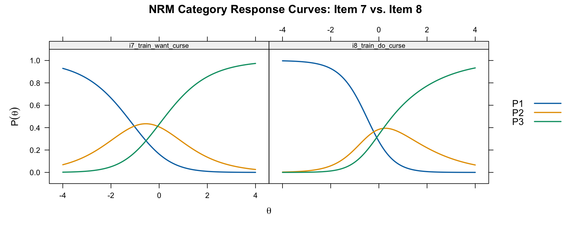

The NRM curves will generally look similar to the GPCM curves for items where the category ordering is confirmed. The NRM is more flexible, however, because it does not impose any ordering constraint.

23.6 General Strategy for Using the NRM

Following the approach from the NRM lecture notes:

1. Fit the model and examine the slope parameters.
2. Check category ordering from the estimated \(a\) values.
3. If ordering is confirmed, the NRM results are consistent with the ordered models (PCM, GPCM, GRM). You can compute Andrich thresholds from the NRM parameters.
4. If ordering is not confirmed, this suggests problems with the category structure for those items.

Note: Just because the \(a\) values are ordered does not guarantee that the thresholds will be ordered (Bock, 1972).

24 Summary

24.1 Models at a Glance

summary_df <- data.frame(
  Model = c("PCM", "GPCM", "RSM", "GRM", "NRM"),
  Family = c("Adjacent", "Adjacent", "Adjacent", "Cumulative", "Nominal"),
  Discrimination = c("Fixed (=1)", "Item-specific", "Fixed (=1)",
                      "Item-specific", "Category-specific"),
  Thresholds = c("Item-specific", "Item-specific", "Common across items",
                  "Item-specific", "Not directly estimated"),
  `Threshold Type` = c("Andrich", "Andrich", "Andrich",
                        "Thurstonian", "Derived from a/c"),
  `Reversals Possible` = c("Yes", "Yes", "Yes", "No (by construction)", "N/A"),
  `Sufficient Statistics` = c("Yes", "No", "Yes", "No", "No"),
  check.names = FALSE
)
knitr::kable(summary_df, caption = "Comparison of Polytomous IRT Models")

Comparison of Polytomous IRT Models

Model	Family	Discrimination	Thresholds	Threshold Type	Reversals Possible	Sufficient Statistics
PCM	Adjacent	Fixed (=1)	Item-specific	Andrich	Yes	Yes
GPCM	Adjacent	Item-specific	Item-specific	Andrich	Yes	No
RSM	Adjacent	Fixed (=1)	Common across items	Andrich	Yes	Yes
GRM	Cumulative	Item-specific	Item-specific	Thurstonian	No (by construction)	No
NRM	Nominal	Category-specific	Not directly estimated	Derived from a/c	N/A	No

24.2 Guidelines for Model Selection

1. Start with the PCM if you have no strong prior about item discrimination. The PCM is the most flexible Rasch-family model and allows you to examine threshold ordering as a diagnostic tool.

2. Try the RSM if all items share the same response format. Test whether the RSM constraint holds using a likelihood ratio test against the PCM.

3. Use the GPCM or GRM if there is evidence that items differ substantially in discrimination and you are willing to give up sufficient statistics. Remember that the GPCM thresholds are Andrich thresholds; the GRM is a cumulative model, so it has Thurstonian thresholds.

4. Use the NRM to empirically test whether response categories are ordered as intended, or when categories are truly nominal.

5. Always examine fit plots — no single fit statistic tells the whole story. Compare category response curves across models to see where they agree and disagree.