---
title: "Deriving and Conceptualizing an Item Characteristic Curve"
author: "Derek C. Briggs and Claude Code (Opus 4.6 & 4.7)"
output:
html_document:
toc: true
toc_float: true
code_folding: show
pdf_document:
toc: true
latex_engine: xelatex
---
```{r inject-rootdir, include=FALSE}
knitr::opts_knit$set(root.dir = "/Users/briggsd/Library/CloudStorage/Dropbox/Github/Measurement and Psychometrics/IRT Models for Dichotomously Scored Items/R Markdown Tutorials")
```
```{r setup, include=FALSE}
knitr::opts_chunk$set(echo = TRUE, message = FALSE, warning = FALSE)
```
## Introduction
This document provides a conceptual derivation of the Item Characteristic Curve (ICC) using the normal ogive. The presentation follows the narrative found in Lord & Novick (1968, pp. 370-371) and Thissen & Orlando (2001, pp. 84-87).
As Lord and Novick wrote:
> "[The equation] may be taken simply as a basic assumption, the utility of which can be investigated for a given set of data (albeit with considerable difficulty). Alternatively [this equation] can be inferred from other, possibly more plausible assumptions. We shall outline one way of doing this, a way that some theorists find interesting and others do not." (Lord & Novick, 1968, p. 370)
---
## Part 1: Statistical Background
Before deriving the ICC, we need to review some foundational concepts about random variables and probability distributions.
### Random Variables and Probability Functions
A **random variable** can be loosely defined as a quantity that can have more than one realized value such that the possible values can be assigned to a probability function.
**Notation conventions:**
- Random variables are denoted using upper case italicized letters: $X$, $Y$, $Z$
- Realized/observed values are denoted using lower case italicized letters: $x$, $y$, $z$
- If we write $P(X=x)=.5$, this says "the probability that random variable $X$ equals the value $x$ is 0.5"
There are two kinds of random variables:
- **Discrete**: Can only take on specific, countable values
- **Continuous**: Can take on any value within a range
### Probability Distribution Functions (pdf)
A probability function provides information about the distribution of a random variable.
#### For Discrete Random Variables
$$p(x) = P(X = x)$$
where:
1. $p(x) \geq 0$ (probabilities must be non-negative)
2. $\sum_{x} p(x) = 1$ (probabilities must sum to 1)
#### For Continuous Random Variables
We represent the pdf as a function $f(x)$ where:
$$P(a \leq X \leq b) = \int_{a}^{b} f(x) \, dx$$
Properties:
1. $f(x) \geq 0$ for $-\infty < x < +\infty$
2. $\int_{-\infty}^{+\infty} f(x) \, dx = 1$
3. $P(X = c) = 0$ (probability of any exact value is 0)
### Cumulative Distribution Functions (cdf)
The cumulative distribution function tells us $P(X \leq x)$.
#### For Discrete Random Variables
$$F(x) = P(X \leq x) = \sum_{t \mid t \leq x} p(t)$$
#### For Continuous Random Variables
$$F(x) = P(X \leq x) = \int_{-\infty}^{x} f(t) \, dt$$
**Key relationship:** To go from a cdf to a pdf, take the first derivative:
$$f(x) = \frac{dF(x)}{dx}$$
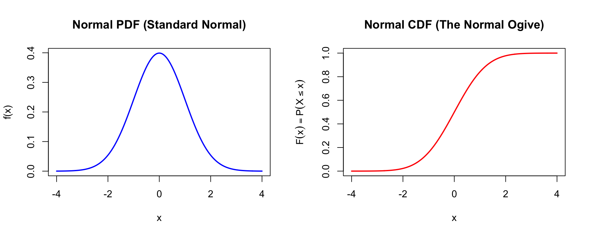
### The Normal (Gaussian) Distribution
The pdf of the normal distribution is:
$$f(x) = \frac{1}{\sqrt{2\pi}\sigma} \exp\left(\frac{-(x-\mu)^2}{2\sigma^2}\right)$$
The cdf (also called the **normal ogive**) is:
$$F(x) = P(X \leq x) = \frac{1}{\sqrt{2\pi}\sigma} \int_{-\infty}^{x} \exp\left(\frac{-(t-\mu)^2}{2\sigma^2}\right) dt$$
```{r normal-plots, fig.width=10, fig.height=4}
par(mfrow = c(1, 2))

# Normal PDF
x <- seq(-4, 4, 0.01)
plot(x, dnorm(x), type = "l", lwd = 2, col = "blue",
     main = "Normal PDF (Standard Normal)",
     xlab = "x", ylab = "f(x)")

# Normal CDF (the "ogive")
plot(x, pnorm(x), type = "l", lwd = 2, col = "red",
     main = "Normal CDF (The Normal Ogive)",
     xlab = "x", ylab = expression(F(x) == P(X <= x)))
par(mfrow = c(1, 1))
```
---
## Part 2: Building the Model
### It Starts with a Test and an Item
Consider the first item on a math test for 6th graders:
> A penny is tossed 20 times. Which of the following is most likely to be the number of times heads came up?
>
> A. 0
> B. 2
> C. 5
> D. 8
> E. 15
This item is trying to find out whether the student has a basic understanding of probability.
### The Response Process Continuum
We assume there is a "response process" continuum that governs whether any individual will answer this item correctly (see Thissen & Orlando, 2001, p. 85).
- This process is represented by the continuous quantity $V_i$ for item $i$
- Each item on the test is associated with a distinct response process quantity $V_i$
- Let $\theta$ represent the general unidimensional construct of "mathematical ability"
- We assume both $V_i$ and $\theta$ have been standardized (mean = 0, SD = 1)
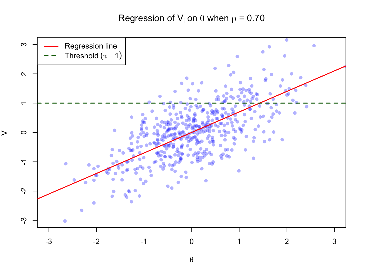
### A Regression Equation
The latent variable underlying any single item can be related to $\theta$ with the linear regression equation:
$$V_i = \rho_i \theta + \varepsilon_i$$
where:
- $\rho_i$ represents the correlation between $V_i$ and $\theta$ (this is a **biserial correlation**)
- $\varepsilon_i$ represents a random error term, where $\varepsilon_i \sim N(0, 1)$
- By construction, $\varepsilon_i$ and $\theta$ are independent
```{r regression-viz, fig.width=8, fig.height=6}
set.seed(123)
n <- 500
rho <- 0.70

# Generate data
theta <- rnorm(n, 0, 1)
epsilon <- rnorm(n, 0, sqrt(1 - rho^2))
V <- rho * theta + epsilon

# Plot
plot(theta, V, pch = 16, col = rgb(0, 0, 1, 0.3),
     xlab = expression(theta), ylab = expression(V[i]),
     main = expression(paste("Regression of ", V[i], " on ", theta, " when ", rho, " = 0.70")),
     xlim = c(-3, 3), ylim = c(-3, 3))
abline(a = 0, b = rho, col = "red", lwd = 2)
abline(h = 1, col = "darkgreen", lwd = 2, lty = 2)
legend("topleft", legend = c("Regression line", expression(Threshold ~ (tau == 1))),
       col = c("red", "darkgreen"), lwd = 2, lty = c(1, 2))
```
### Key Properties
The regression line predicts the conditional mean of $V_i$ given $\theta$:
$$E(V_i | \theta) = \rho_i \theta$$
The conditional standard deviation (RMSE) is:
$$\sigma_{\varepsilon|\theta} = \sqrt{1 - \rho_i^2}$$
The distribution of $V_i | \theta$ is assumed to be normal.
---
## Part 3: Deriving the ICC
### Using the Normal CDF
Given a threshold $\tau_i$ for item $i$, we want to find:
$$P(V_i > \tau_i | \theta)$$
This is calculated using the conditional normal cdf:
$$P(V_i \leq \tau_i | \theta) = \frac{1}{\sqrt{2\pi}\sigma_{\varepsilon|\theta}} \int_{-\infty}^{\tau_i} \exp\left(\frac{-(t - E(V_i|\theta))^2}{2\sigma_{\varepsilon|\theta}^2}\right) dt$$
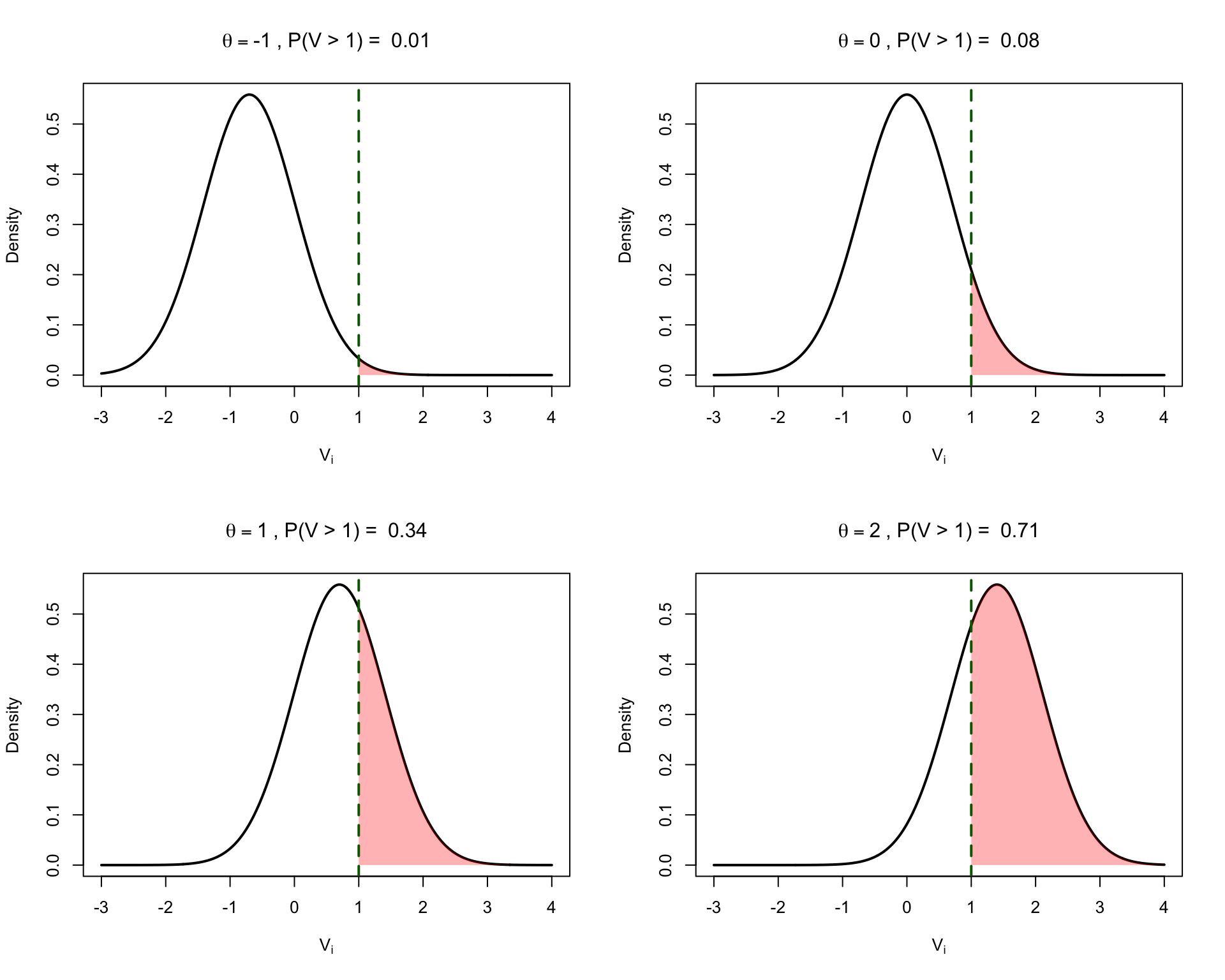
### Example Calculations
Let $\rho_i = 0.70$ and $\tau_i = 1$.
Then $\sigma_{\varepsilon|\theta} = \sqrt{1 - 0.70^2} = \sqrt{0.51} \approx 0.71$
```{r example-calcs}
rho <- 0.70
tau <- 1
sigma_eps <- sqrt(1 - rho^2)

# For different values of theta
theta_vals <- c(-1, 0, 1, 2)

for (th in theta_vals) {
  E_V <- rho * th
  prob <- 1 - pnorm(tau, mean = E_V, sd = sigma_eps)
  cat(sprintf("When θ = %2d: E(V|θ) = %5.2f, P(V > τ|θ) = %.3f\n", th, E_V, prob))
}
```
### Visualizing the Probability Calculation
```{r prob-visualization, fig.width=10, fig.height=8}
par(mfrow = c(2, 2))

theta_vals <- c(-1, 0, 1, 2)
v_range <- seq(-3, 4, 0.01)

for (th in theta_vals) {
  E_V <- rho * th
  prob <- 1 - pnorm(tau, mean = E_V, sd = sigma_eps)

  # Plot the conditional distribution
  plot(v_range, dnorm(v_range, mean = E_V, sd = sigma_eps), type = "l", lwd = 2,
       xlab = expression(V[i]), ylab = "Density",
       main = bquote(theta == .(th) ~ ", P(V > 1) = " ~ .(round(prob, 2))))

  # Shade the area above threshold
  v_above <- v_range[v_range >= tau]
  polygon(c(tau, v_above, max(v_above)),
          c(0, dnorm(v_above, mean = E_V, sd = sigma_eps), 0),
          col = rgb(1, 0, 0, 0.3), border = NA)

  abline(v = tau, col = "darkgreen", lwd = 2, lty = 2)
}
par(mfrow = c(1, 1))
```
### From Latent to Observed
Both $V_i$ and $\theta$ are latent variables. We link the observed item response to $\theta$ through a **dichotomization rule**:
Let $X_i$ be a discrete random variable representing the observed response to item $i$:
- If $V_i > \tau_i$ then $X_i = 1$ (correct)
- If $V_i \leq \tau_i$ then $X_i = 0$ (incorrect)
This implies:
$$P(X_i = 1 | \theta) = P(V_i > \tau_i | \theta)$$
---
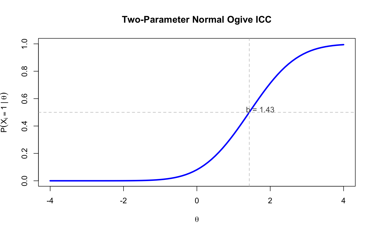
## Part 4: The Two-Parameter Normal Ogive Model
Putting this all together, we can write:
$$P(X_i = 1 | \theta) = \Phi(a_i(\theta - b_i))$$
where $\Phi$ is the standard normal cdf, and:
$$a_i = \frac{\rho_i}{\sqrt{1 - \rho_i^2}} \quad \text{(discrimination)}$$
$$b_i = \frac{\tau_i}{\rho_i} \quad \text{(difficulty)}$$
### Example
Given $\rho_i = 0.70$ and $\tau_i = 1$:
```{r param-conversion}
rho <- 0.70
tau <- 1

a <- rho / sqrt(1 - rho^2)
b <- tau / rho

cat(sprintf("Discrimination (a) = %.2f\n", a))
cat(sprintf("Difficulty (b) = %.2f\n", b))
```
### Plotting the ICC
```{r icc-plot, fig.width=8, fig.height=5}
theta <- seq(-4, 4, 0.1)
prob <- pnorm(a * (theta - b))

plot(theta, prob, type = "l", lwd = 3, col = "blue",
     xlab = expression(theta), ylab = expression(P(X[i] == 1 ~ "|" ~ theta)),
     main = "Two-Parameter Normal Ogive ICC",
     ylim = c(0, 1))
abline(h = 0.5, lty = 2, col = "gray")
abline(v = b, lty = 2, col = "gray")
text(b + 0.3, 0.52, paste("b =", round(b, 2)), col = "gray30")
```
### Interpretation of Parameters
This derivation explains why:
1. The **discrimination parameter** ($a_i$) in the 2PL IRT model is analogous to the correlation between the item and the construct of measurement
2. The **difficulty parameter** ($b_i$) is analogous to the threshold between a correct and incorrect response (inversely related to the proportion answering correctly)
### Converting Between Parameterizations
To go from IRT parameters back to factor analytic parameters:
$$\rho_i = \frac{a_i}{\sqrt{1 + a_i^2}} \quad \text{(biserial correlation / factor loading)}$$
$$\tau_i = b_i \cdot \rho_i \quad \text{(threshold)}$$
*Note: These relationships only hold if $\theta$ is normally distributed and there is no guessing on items.*
---
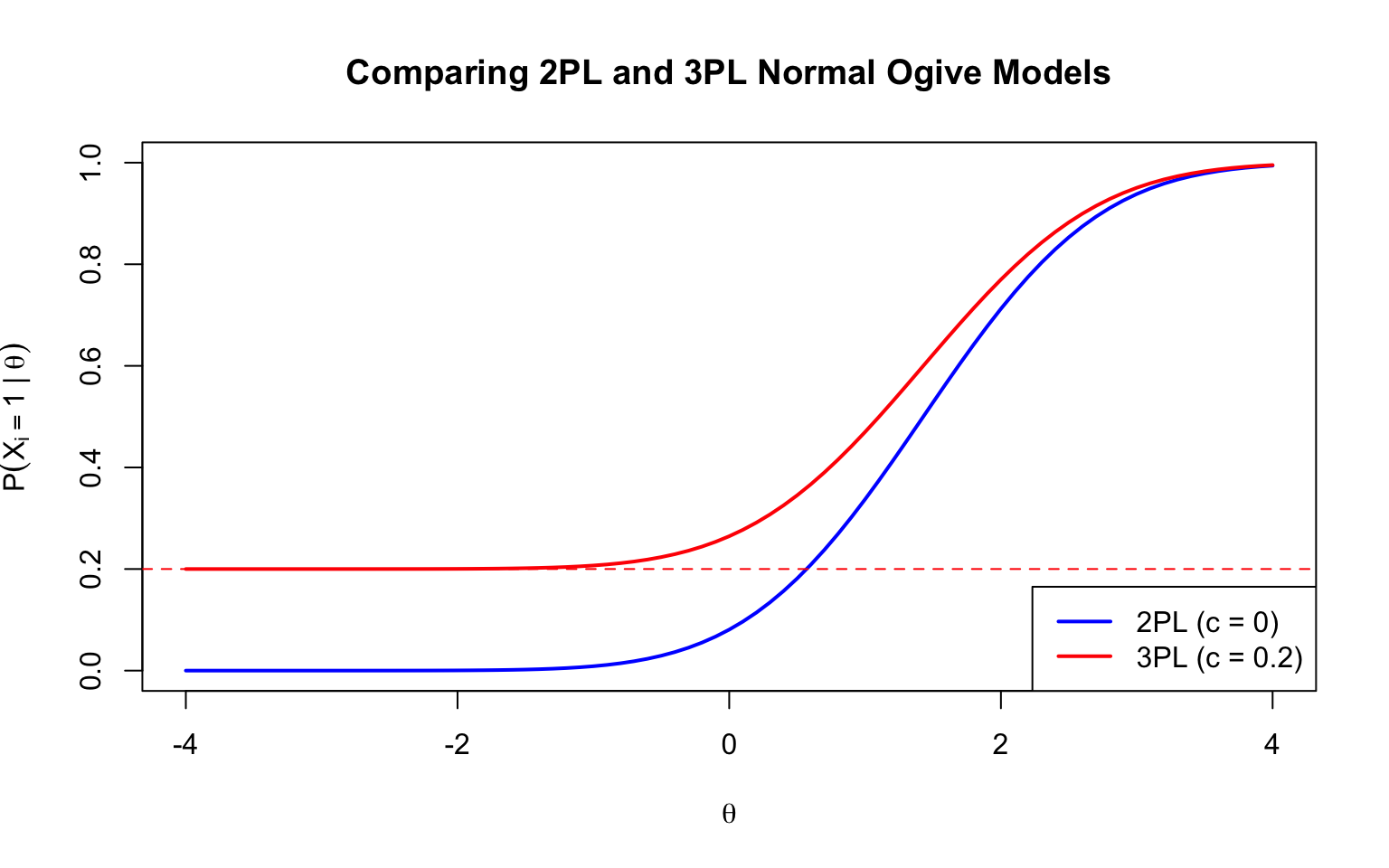
## Part 5: The Three-Parameter Normal Ogive Model
Adding a lower asymptote (guessing parameter):
$$P(X_i = 1 | \theta, b_i, a_i, c_i) = c_i + (1 - c_i) \Phi(a_i(\theta - b_i))$$
where $c_i$ represents the probability of a correct response by guessing.
```{r three-param, fig.width=8, fig.height=5}
theta <- seq(-4, 4, 0.1)
c_param <- 0.20  # guessing parameter

prob_2pl <- pnorm(a * (theta - b))
prob_3pl <- c_param + (1 - c_param) * pnorm(a * (theta - b))

plot(theta, prob_2pl, type = "l", lwd = 2, col = "blue",
     xlab = expression(theta), ylab = expression(P(X[i] == 1 ~ "|" ~ theta)),
     main = "Comparing 2PL and 3PL Normal Ogive Models",
     ylim = c(0, 1))
lines(theta, prob_3pl, lwd = 2, col = "red")
abline(h = c_param, lty = 2, col = "red")
legend("bottomright", legend = c("2PL (c = 0)", paste0("3PL (c = ", c_param, ")")),
       col = c("blue", "red"), lwd = 2)
```
---
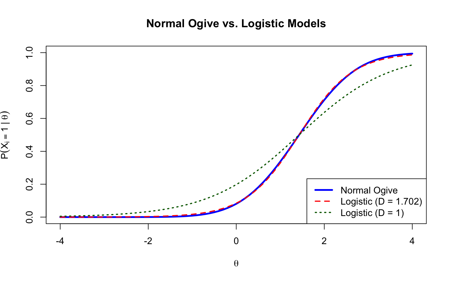
## Part 6: The Logistic Approximation
The logistic distribution provides a close approximation to the normal distribution and is computationally simpler.
### Logistic vs. Normal Ogive
The logistic IRT model can be written as:
$$P(X_i = 1 | \theta) = c_i + (1 - c_i) \frac{\exp(Da_i(\theta - b_i))}{1 + \exp(Da_i(\theta - b_i))}$$
where $D = 1.702$ makes the logistic model approximately equal to the normal ogive model.
```{r logistic-comparison, fig.width=8, fig.height=5}
theta <- seq(-4, 4, 0.1)
D <- 1.702

# Normal ogive
prob_normal <- pnorm(a * (theta - b))

# Logistic with D scaling
prob_logistic_D <- plogis(D * a * (theta - b))

# Logistic without D scaling
prob_logistic <- plogis(a * (theta - b))

plot(theta, prob_normal, type = "l", lwd = 3, col = "blue",
     xlab = expression(theta), ylab = expression(P(X[i] == 1 ~ "|" ~ theta)),
     main = "Normal Ogive vs. Logistic Models",
     ylim = c(0, 1))
lines(theta, prob_logistic_D, lwd = 2, col = "red", lty = 2)
lines(theta, prob_logistic, lwd = 2, col = "darkgreen", lty = 3)
legend("bottomright",
       legend = c("Normal Ogive", "Logistic (D = 1.702)", "Logistic (D = 1)"),
       col = c("blue", "red", "darkgreen"), lwd = c(3, 2, 2), lty = c(1, 2, 3))
```
### Modern Practice
Historically, researchers used the $D = 1.702$ scaling to make logistic parameters match normal ogive parameters. Today, most practitioners simply use the logistic version without $D$ because:
1. The logistic is easier to estimate
2. There isn't much practical need to match normal ogive parameters
3. Model fit is essentially the same
---
## Summary
1. The ICC can be derived by conceptualizing a latent response process continuum $V_i$ that underlies observed item responses
2. The regression of $V_i$ on $\theta$ with a threshold dichotomization rule leads to the normal ogive model
3. The discrimination parameter $a_i$ reflects how strongly the item relates to the construct
4. The difficulty parameter $b_i$ reflects the threshold for a correct response
5. The logistic model provides a computationally convenient approximation to the normal ogive
---
## References
Lord, F. M., & Novick, M. R. (1968). *Statistical theories of mental test scores*. Addison-Wesley.
Thissen, D., & Orlando, M. (2001). Item response theory for items scored in two categories. In D. Thissen & H. Wainer (Eds.), *Test scoring* (pp. 73-140). Lawrence Erlbaum Associates.