---
title: "Test Characteristic Curves, Information Functions, and SEM"
author: "Derek C. Briggs and Claude Code (Opus 4.6 & 4.7)"
output:
html_document:
toc: true
toc_float: true
code_folding: show
pdf_document:
toc: true
latex_engine: xelatex
---
```{r inject-rootdir, include=FALSE}
knitr::opts_knit$set(root.dir = "/Users/briggsd/Library/CloudStorage/Dropbox/Github/Measurement and Psychometrics/IRT Models for Dichotomously Scored Items/R Markdown Tutorials")
```
```{r setup, include=FALSE}
knitr::opts_chunk$set(echo = TRUE, message = FALSE, warning = FALSE)
```
## Introduction
This document covers three important concepts in IRT:
1. **Test Characteristic Curves (TCC)**: The expected test score as a function of ability
2. **Information Functions**: How much "information" items and tests provide about ability
3. **Standard Error of Measurement (SEM)**: The precision of ability estimates
---
## Part 1: Test Characteristic Curves
### Expected Item Response
For a dichotomously scored item, the expected value of a respondent's answer is:
$$E(X_{ip} | \theta_p) = P(X_{ip} = 1 | \theta_p) = P_i(\theta)$$
Because $X_{ip}$ is a binary variable (0 or 1), the mean equals the probability.
This means: of all people with ability $\theta_p$, we expect $P_i(\theta_p)$ proportion to get the item right.
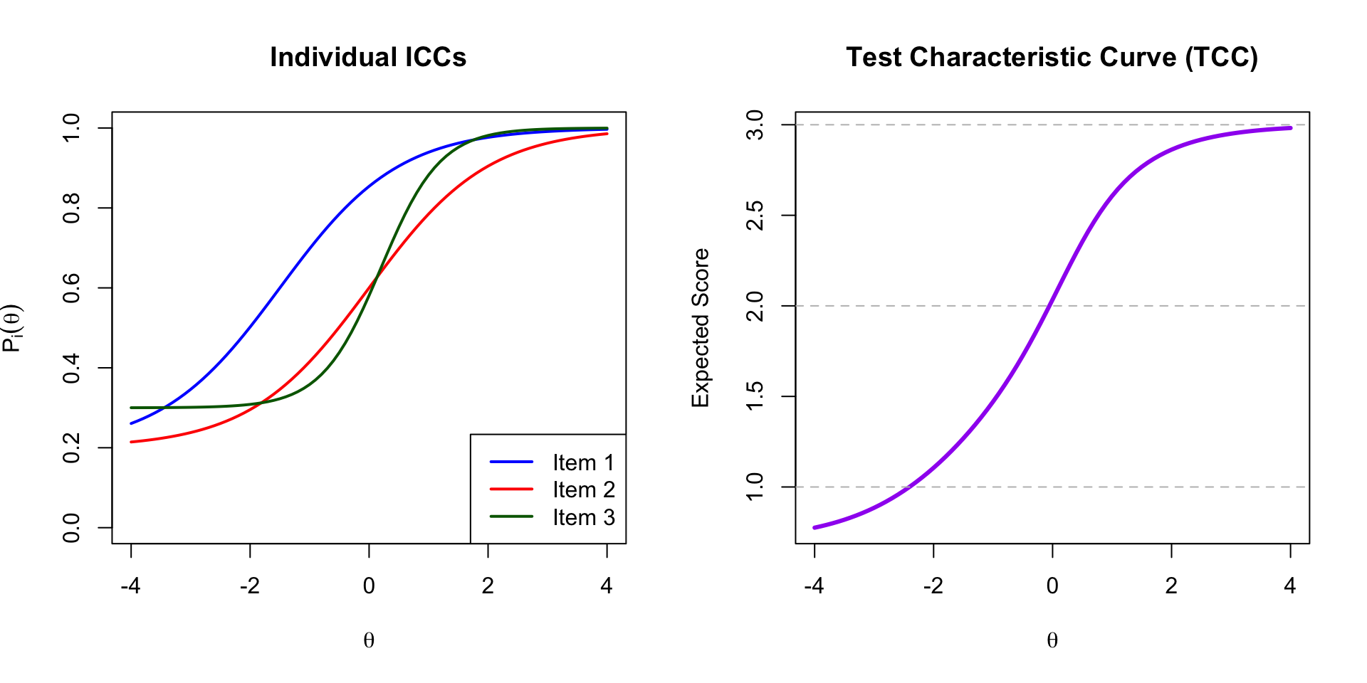
### Expected Test Score: The TCC
The expected observed (number correct) score for a person can be calculated by summing the ICCs across items:
$$TCC(\theta_p) = \sum_{i=1}^{I} P_i(\theta_p)$$
This **Test Characteristic Curve** tells us the expected number of correct answers for each level of theta.
We can think of this as an estimate of the true score associated with a particular set of items.
### Example: Three-Item Test
```{r tcc-functions}
# 3PL probability function
calc_prob <- function(theta, a, b, c) {
  c + (1 - c) * exp(a * (theta - b)) / (1 + exp(a * (theta - b)))
}

# Item parameters (from three_item_test.xlsx)
items <- data.frame(
  item = 1:3,
  a = c(1, 1, 2),
  b = c(-1.5, 0, 0.2),
  c = c(0.2, 0.2, 0.3)
)

knitr::kable(items, caption = "Item Parameters")
```
```{r tcc-plot, fig.width=10, fig.height=5}
theta <- seq(-4, 4, 0.1)

# Calculate individual ICCs
p1 <- calc_prob(theta, items$a[1], items$b[1], items$c[1])
p2 <- calc_prob(theta, items$a[2], items$b[2], items$c[2])
p3 <- calc_prob(theta, items$a[3], items$b[3], items$c[3])

# Calculate TCC (sum of probabilities)
tcc <- p1 + p2 + p3

par(mfrow = c(1, 2))

# Plot individual ICCs
plot(theta, p1, type = "l", lwd = 2, col = "blue",
     xlab = expression(theta), ylab = expression(P[i](theta)),
     main = "Individual ICCs", ylim = c(0, 1))
lines(theta, p2, lwd = 2, col = "red")
lines(theta, p3, lwd = 2, col = "darkgreen")
legend("bottomright", legend = paste("Item", 1:3),
       col = c("blue", "red", "darkgreen"), lwd = 2)

# Plot TCC
plot(theta, tcc, type = "l", lwd = 3, col = "purple",
     xlab = expression(theta), ylab = "Expected Score",
     main = "Test Characteristic Curve (TCC)")
abline(h = c(0, 1, 2, 3), lty = 2, col = "gray")
par(mfrow = c(1, 1))
```
**Interpretation:**
- At $\theta = -4$: Expected score $\approx$ `r round(tcc[theta == -4], 2)` (mostly guessing)
- At $\theta = 0$: Expected score $\approx$ `r round(tcc[theta == 0], 2)`
- At $\theta = 4$: Expected score $\approx$ `r round(tcc[theta == 4], 2)` (nearly all correct)
---
## Part 2: Item Information Functions
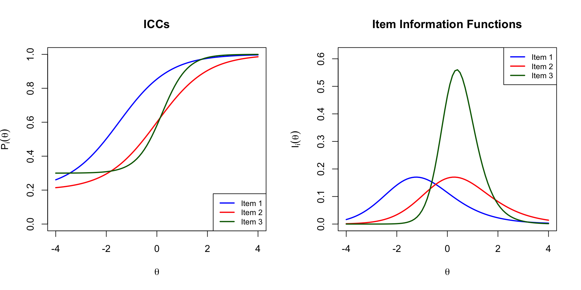
### What is "Information"?
Each item provides a certain amount of "information" about respondents' ability levels. The item information function is:
$$I_i(\theta) = \frac{[P'_i(\theta)]^2}{P_i(\theta) Q_i(\theta)}$$
where:
- $P_i(\theta) = P(X_{ip} = 1 | \theta_p)$
- $Q_i(\theta) = 1 - P_i(\theta)$
- $P'_i(\theta)$ is the first derivative of $P_i(\theta)$
**Key insight:** Items provide different amounts of information at different points on the theta scale.
### Model-Specific Information Functions
| Model | Item Information Formula | Maximum At |
|:------|:------------------------|:-----------|
| 1PL | $P_i(\theta) Q_i(\theta)$ | $b_i$ |
| 2PL | $a_i^2 P_i(\theta) Q_i(\theta)$ | $b_i$ |
| 3PL | $\frac{a_i^2 Q_i(\theta)}{P_i(\theta)} \cdot \frac{[P_i(\theta) - c_i]^2}{(1-c_i)^2}$ | Slightly above $b_i$ |
### Computing Item Information
```{r item-info-function}
# 3PL item information function
calc_info <- function(theta, a, b, c) {
  # Calculate P and Q
  L <- 1 / (1 + exp(-a * (theta - b)))
  P <- c + (1 - c) * L
  Q <- 1 - P

  # Calculate derivative of P
  dP <- (1 - c) * a * L * (1 - L)

  # Information
  info <- (dP^2) / (P * Q)
  return(info)
}
```
```{r item-info-plot, fig.width=10, fig.height=5}
# Calculate item information for each item
info1 <- calc_info(theta, items$a[1], items$b[1], items$c[1])
info2 <- calc_info(theta, items$a[2], items$b[2], items$c[2])
info3 <- calc_info(theta, items$a[3], items$b[3], items$c[3])

par(mfrow = c(1, 2))

# Plot ICCs
plot(theta, p1, type = "l", lwd = 2, col = "blue",
     xlab = expression(theta), ylab = expression(P[i](theta)),
     main = "ICCs", ylim = c(0, 1))
lines(theta, p2, lwd = 2, col = "red")
lines(theta, p3, lwd = 2, col = "darkgreen")
legend("bottomright", legend = paste("Item", 1:3),
       col = c("blue", "red", "darkgreen"), lwd = 2, cex = 0.8)

# Plot Item Information
plot(theta, info1, type = "l", lwd = 2, col = "blue",
     xlab = expression(theta), ylab = expression(I[i](theta)),
     main = "Item Information Functions",
     ylim = c(0, max(c(info1, info2, info3)) * 1.1))
lines(theta, info2, lwd = 2, col = "red")
lines(theta, info3, lwd = 2, col = "darkgreen")
legend("topright", legend = paste("Item", 1:3),
       col = c("blue", "red", "darkgreen"), lwd = 2, cex = 0.8)
par(mfrow = c(1, 1))
```
**Observations:**
- Item 3 (green) has the highest peak information because it has the highest discrimination ($a = 2$)
- Information is maximized near each item's difficulty parameter ($b$)
- Items with higher discrimination provide more information but over a narrower range
---
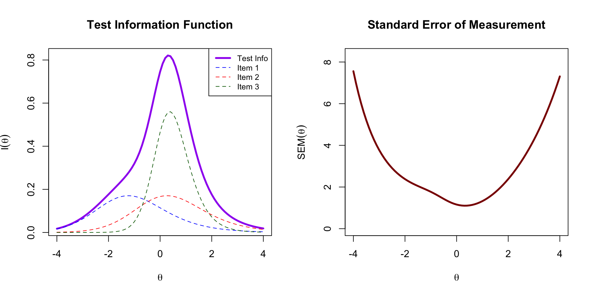
## Part 3: Test Information Function
### Summing Item Information
The test information function is calculated by summing the item information functions:
$$I(\theta) = \sum_{i=1}^{I} I_i(\theta)$$
### Relationship to SEM
The standard error of measurement for theta is:
$$SEM(\theta) = \frac{1}{\sqrt{I(\theta)}}$$
**Key relationships:**
- As information **increases**, SEM **decreases**
- $SEM(\theta)$ **varies** across the theta distribution
- Tests provide more precise estimates where they have more information
```{r test-info, fig.width=10, fig.height=5}
# Calculate test information
test_info <- info1 + info2 + info3

# Calculate SEM
sem <- 1 / sqrt(test_info)

par(mfrow = c(1, 2))

# Plot Test Information
plot(theta, test_info, type = "l", lwd = 3, col = "purple",
     xlab = expression(theta), ylab = expression(I(theta)),
     main = "Test Information Function")

# Also show individual item contributions
lines(theta, info1, lwd = 1, col = "blue", lty = 2)
lines(theta, info2, lwd = 1, col = "red", lty = 2)
lines(theta, info3, lwd = 1, col = "darkgreen", lty = 2)
legend("topright",
       legend = c("Test Info", "Item 1", "Item 2", "Item 3"),
       col = c("purple", "blue", "red", "darkgreen"),
       lwd = c(3, 1, 1, 1), lty = c(1, 2, 2, 2), cex = 0.8)

# Plot SEM
plot(theta, sem, type = "l", lwd = 3, col = "darkred",
     xlab = expression(theta), ylab = expression(SEM(theta)),
     main = "Standard Error of Measurement",
     ylim = c(0, max(sem[is.finite(sem)]) * 1.1))
par(mfrow = c(1, 1))
```
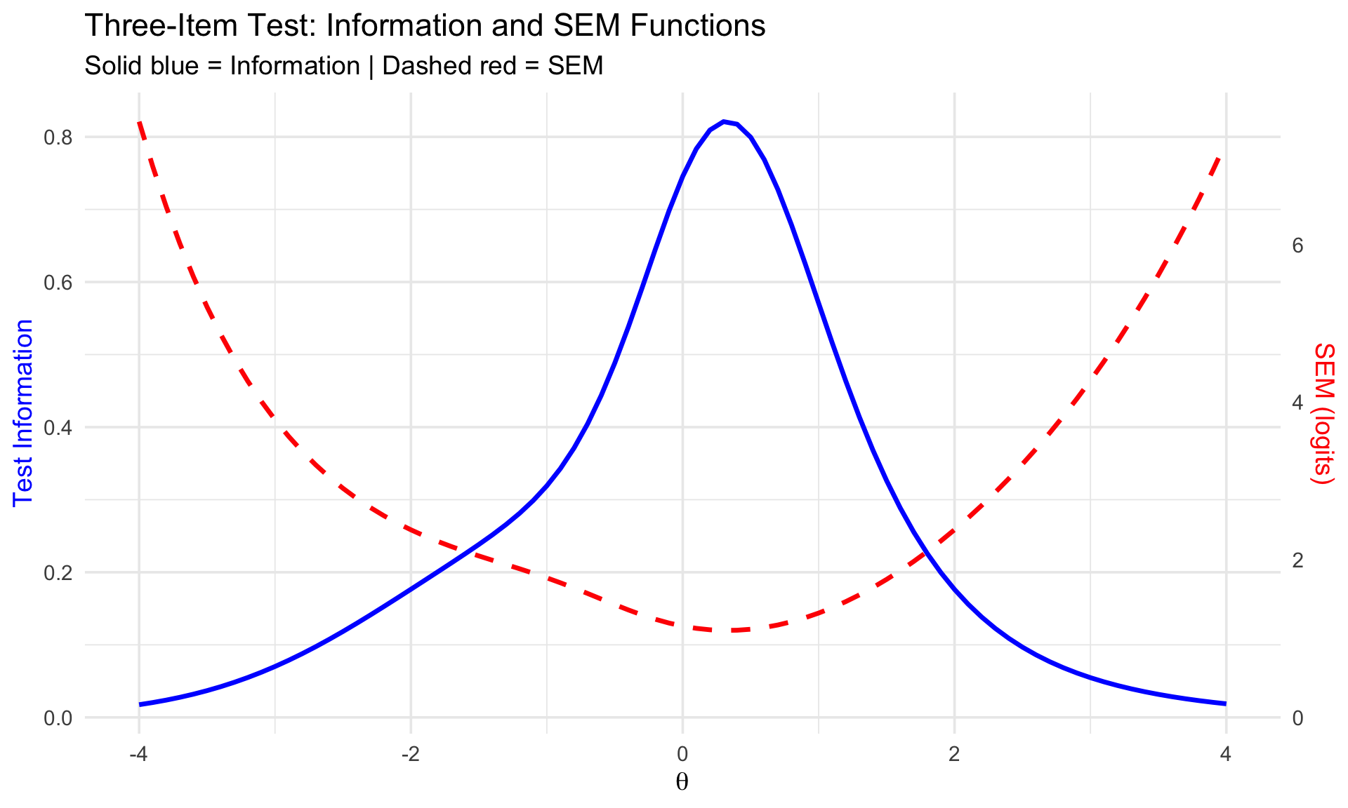
### Combined Plot: Information and SEM
```{r info-sem-dual, fig.width=10, fig.height=6}
library(ggplot2)

# Create data frame
plot_df <- data.frame(
  theta = theta,
  info = test_info,
  sem = sem
)

# Scale factor for dual axis
scale_factor <- max(plot_df$info, na.rm = TRUE) / max(plot_df$sem[is.finite(plot_df$sem)], na.rm = TRUE)
plot_df$sem_scaled <- plot_df$sem * scale_factor

# Dual-axis plot
ggplot(plot_df, aes(x = theta)) +
  geom_line(aes(y = info), linewidth = 1.2, color = "blue") +
  geom_line(aes(y = sem_scaled), linewidth = 1.2, linetype = "dashed", color = "red") +
  scale_y_continuous(
    name = "Test Information",
    sec.axis = sec_axis(~ . / scale_factor, name = "SEM (logits)")
  ) +
  labs(
    x = expression(theta),
    title = "Three-Item Test: Information and SEM Functions",
    subtitle = "Solid blue = Information | Dashed red = SEM"
  ) +
  theme_minimal(base_size = 14) +
  theme(
    axis.title.y.left = element_text(color = "blue"),
    axis.title.y.right = element_text(color = "red")
  )
```
**Interpretation:**
- The test provides maximum information (minimum SEM) around $\theta \approx 0$
- At the extremes ($\theta < -2$ or $\theta > 2$), information drops and SEM increases
- This three-item test measures best in the middle of the ability range
---
## Part 4: Practice with Real Data Using mirt
Now let's apply these concepts to real data using the `mirt` package.
```{r load-packages}
library(mirt)
```
### Load Data and Fit Model
```{r fit-model, results='hide'}
# Load data
forma <- read.csv("../Data/pset1_formA.csv")
forma <- forma[, 1:15]

# Fit 2PL model
mirt_2pl <- mirt(forma, model = 1, itemtype = "2PL", method = "EM")
```
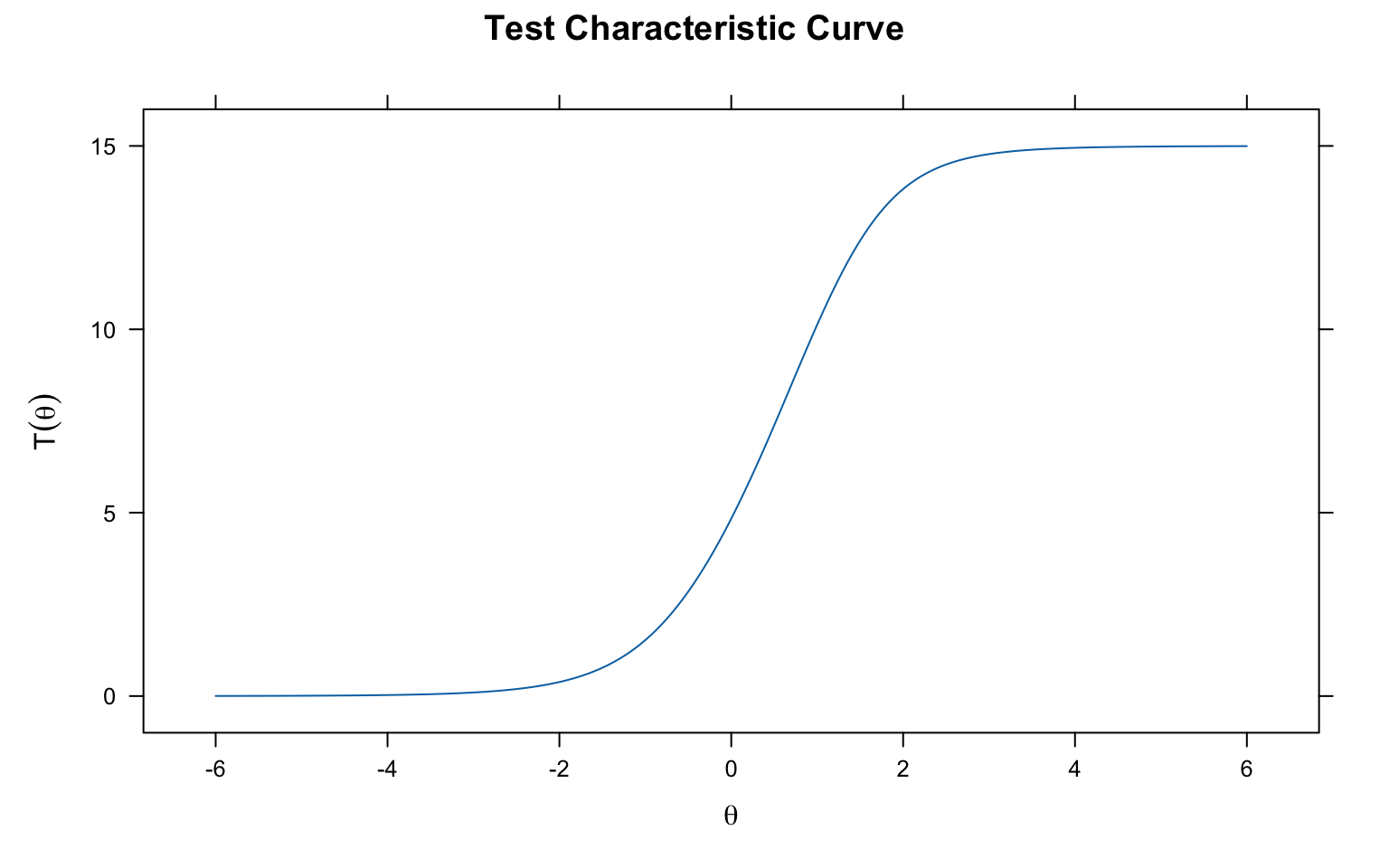
### Test Characteristic Curve
```{r mirt-tcc, fig.width=8, fig.height=5}
plot(mirt_2pl, main = "Test Characteristic Curve")
```
The TCC shows the expected number of correct answers (out of 15) at each ability level.
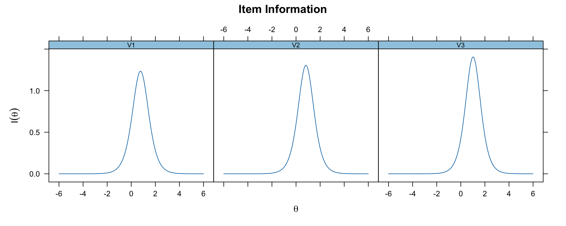
### Item Information Functions
```{r mirt-item-info, fig.width=10, fig.height=4}
# Show item information for first 3 items
plot(mirt_2pl, type = 'infotrace', which.items = 1:3)
```
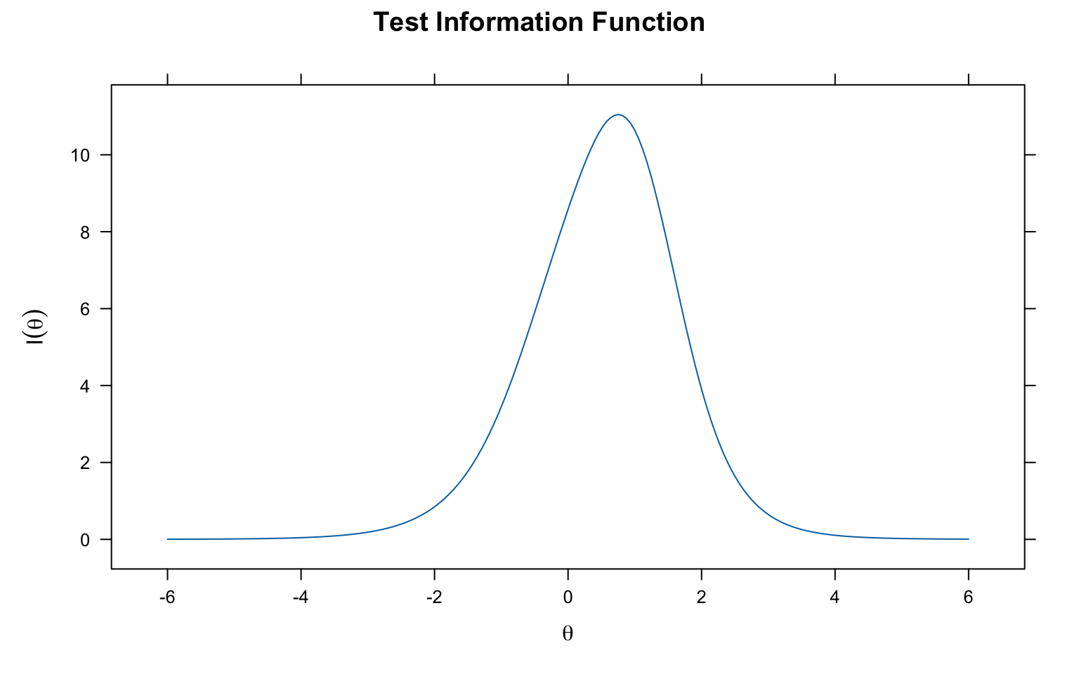
### Test Information Function
```{r mirt-test-info, fig.width=8, fig.height=5}
plot(mirt_2pl, type = 'info', main = "Test Information Function")
```
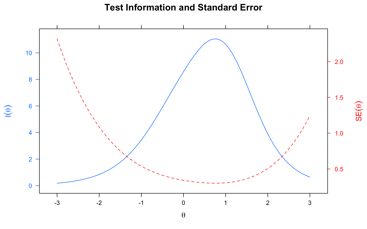
### Test Information and SEM
```{r mirt-info-sem, fig.width=8, fig.height=5}
plot(mirt_2pl, type = 'infoSE', theta_lim = c(-3, 3),
     main = "Test Information and Standard Error")
```
---
## Practical Applications
### Using Information for Test Construction
Item and test information are especially useful for:
1. **Constructing tests**: Select items that provide information where it's needed
2. **Predicting precision**: Know the SEM of theta scores before administering
3. **Targeted measurement**: Increase information at specific points in the theta distribution
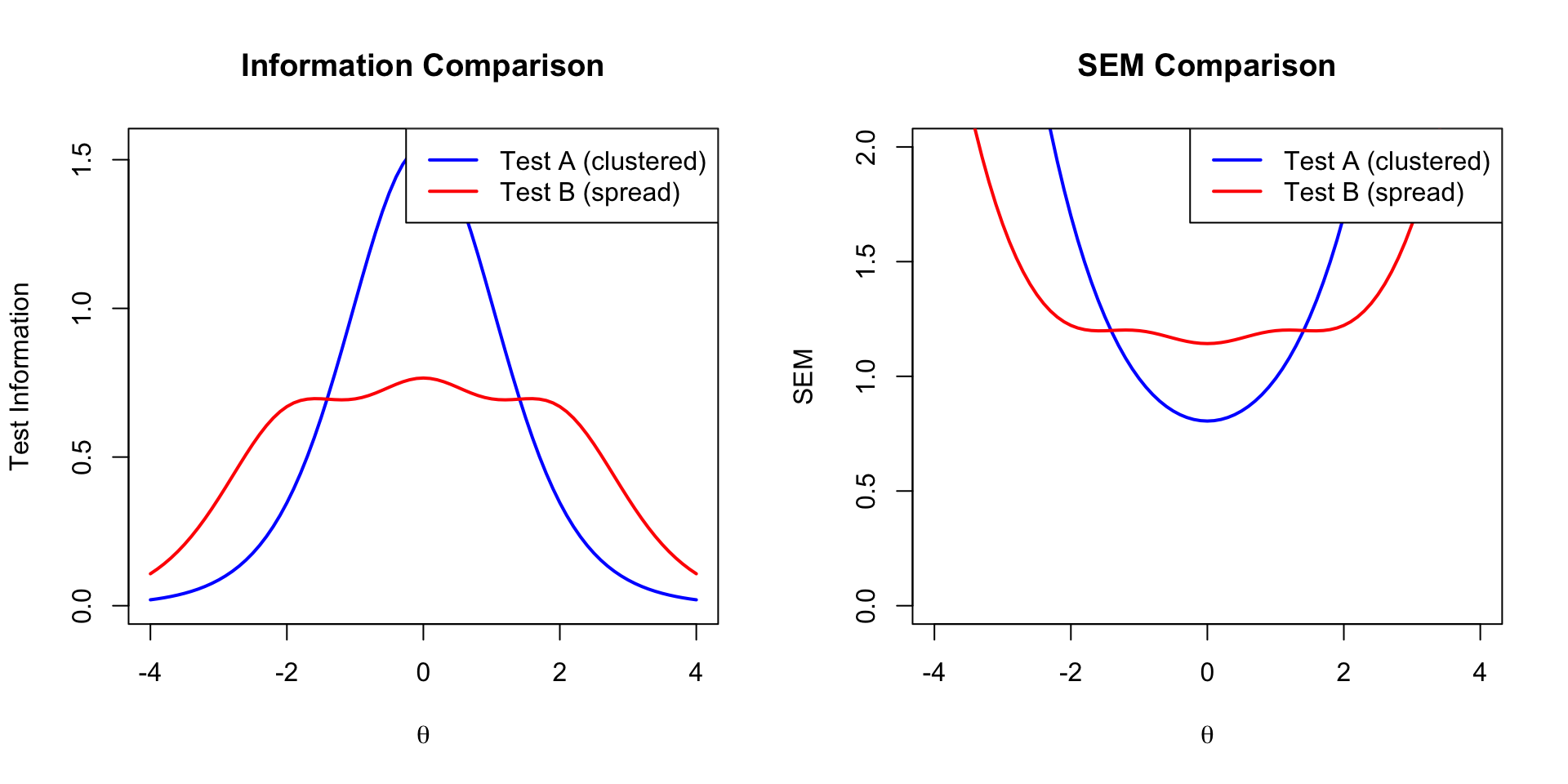
### Example: Comparing Two Tests
```{r test-comparison, fig.width=10, fig.height=5}
# Simulate two different tests
theta <- seq(-4, 4, 0.1)

# Test A: Items clustered around theta = 0
test_a_info <- calc_info(theta, 1.5, -0.5, 0) +
               calc_info(theta, 1.5, 0, 0) +
               calc_info(theta, 1.5, 0.5, 0)

# Test B: Items spread across theta range
test_b_info <- calc_info(theta, 1.5, -2, 0) +
               calc_info(theta, 1.5, 0, 0) +
               calc_info(theta, 1.5, 2, 0)

par(mfrow = c(1, 2))

# Information comparison
plot(theta, test_a_info, type = "l", lwd = 2, col = "blue",
     xlab = expression(theta), ylab = "Test Information",
     main = "Information Comparison", ylim = c(0, max(c(test_a_info, test_b_info))))
lines(theta, test_b_info, lwd = 2, col = "red")
legend("topright", legend = c("Test A (clustered)", "Test B (spread)"),
       col = c("blue", "red"), lwd = 2)

# SEM comparison
sem_a <- 1 / sqrt(test_a_info)
sem_b <- 1 / sqrt(test_b_info)

plot(theta, sem_a, type = "l", lwd = 2, col = "blue",
     xlab = expression(theta), ylab = "SEM",
     main = "SEM Comparison", ylim = c(0, 2))
lines(theta, sem_b, lwd = 2, col = "red")
legend("topright", legend = c("Test A (clustered)", "Test B (spread)"),
       col = c("blue", "red"), lwd = 2)
par(mfrow = c(1, 1))
```
**Conclusion:**
- **Test A** (clustered items): High precision around $\theta = 0$, poor at extremes
- **Test B** (spread items): More uniform precision across the ability range
The choice depends on your measurement goals!
---
## Summary
| Concept | Formula | Key Points |
|:--------|:--------|:-----------|
| TCC | $\sum P_i(\theta)$ | Expected score at each ability level |
| Item Info | $\frac{[P'_i(\theta)]^2}{P_i(\theta)Q_i(\theta)}$ | Varies by item and ability |
| Test Info | $\sum I_i(\theta)$ | Sum of item information |
| SEM | $1/\sqrt{I(\theta)}$ | Inverse relationship with information |
**Key takeaways:**
1. The TCC links ability ($\theta$) to expected test score
2. Items provide maximum information near their difficulty parameter
3. Higher discrimination = more information (but narrower range)
4. Test information determines measurement precision
5. SEM varies across the ability distribution