---
title: "IRT Equating using mirt"
author: "Derek C. Briggs and Claude Code (Opus 4.6 & 4.7)"
output:
html_document:
toc: true
toc_float: true
toc_depth: 3
number_sections: true
code_folding: show
---
```{r inject-rootdir, include=FALSE}
knitr::opts_knit$set(root.dir = "/Users/briggsd/Library/CloudStorage/Dropbox/Github/Measurement and Psychometrics/Test Equating and Linking/R Markdown Tutorials")
```
```{r setup, include=FALSE}
knitr::opts_chunk$set(echo = TRUE, warning = FALSE, message = FALSE)
```
## Introduction
Psychometrcians do **test equating** to ensure that scores from two different forms of a test are comparable, even if one happens to be harder than the other. You might need to do this when administering multiple parallel forms for security reasons (to prevent cheating), or when releasing items each year and replacing them with new ones. In either case, you want scores from one form to carry the same meaning as scores from another form, even though different students took different tests.
---
## Using IRT to Equate Two Test Forms
The way this is typically done in practice when we can't assume that two groups of students have equivalent ability distributions is by embedding some common items in the two test forms. If these items show adequate fit to an IRT model, then they have the property of **parameter invariance**, which means that beyond estimation error they should be the same---up to a linear transformation---regardless of the ability of the students used to calibrate them. We are going to take advantage of this property to use IRT methods to equate two test forms. There are three ways this can be accomplished:
1. Calibrate each test form separately with an IRT model ("separate calibration"), then use the two sets of estimates for the common item parameters shared by the two forms to compute the linking constants needed to express theta values for Form 2 on the scale as theta values for Form 1.
2. Calibrate the items on Form 1, then fix the common items on Form 2 to the values estimated for Form 1. This is known as "anchored calibration."
3. Calibrate all the items on both test forms concurrently ("concurrent calibration") by treating the data as coming from two groups in a single administration, with data on form-specific unique items treated as missing at random.
---
## Simulating a Non-Equivalent Group Anchor Test (NEAT) Design
Let's simulate data from two 20-item test forms that have been collected using a NEAT design such that the first 10 items on each form are the same (anchor items) but the second 10 are unique. There are 20 unique items across the two forms and 10 common items, for 30 distinct items in total. We assume 500 students take each form, with students taking Form 1 having lower ability on average and more variability than students taking Form 2.
Our goal is to express the item and person parameters for form 2 on the scale of form 1. So the "from" scale is form 2 (right hand side of transformation equations that will follow) and the "to" scale (left hand side of transformation equations) is form 1.
### A Disclaimer
I am taking a somewhat "lazy" approach in generating my true item parameters: I am not targeting any known item parameter distributions for an real world test. In practice, item difficulty and discrimination tend to be positively correlated, but I draw values for them independently. This could result in some difficulty and discrimination values for any given item that might be unusual in practice.
Also, the equating literature assumes that for two forms to be candidates for equating, they should have approximately the same reliability. But this is a condition that I'm not enforcing, and as you'll see, I end up simulating two test forms that differ in reliability.
Finally, as I'll show in a separate document, when simulating data from a relatively small number of anchor items (10) with a (relatively) small sample of students taking the items (500), we can get some rather noisy estimates our linking parameters for any given data set, so don't be surprised if we don't recover truth perfectly.
In other words, take the simulated data with a grain of salt; I'm using them for didactic purposes to demonstrate IRT equating using `mirt`.
```{r generate-pars}
library(mirt)
library(dplyr)
library(kableExtra)

# Fixed seed for reproducibility
set.seed(17)

# Item difficulty parameters (IRT b-parameterization)
b1 <- rnorm(20)                        # Form 1: 20 difficulties
b2 <- c(b1[1:10], rnorm(10))          # Form 2: same anchor difficulties + 10 unique

# Item discrimination parameters (IRT a-parameterization)
a1 <- runif(20, .5, 2)
a2 <- c(a1[1:10], runif(10, .5, 2))  # Form 2: same anchor discriminations + 10 unique

# Convert to mirt slope-intercept parameterization
d1 <- -a1 * b1
d2 <- -a2 * b2

# Person ability parameters
th1 <- rnorm(500, 0, 1)       # Group 1: N(0, 1)
th2 <- rnorm(500, .5, .8)     # Group 2: N(0.5, 0.8) -- higher mean, less spread
```
Now we simulate two 500-by-20 matrices of dichotomous item responses using `simdata`.
```{r simulate}
test1 <- as.data.frame(simdata(a = a1, d = d1, Theta = th1, itemtype = 'dich'))
test2 <- as.data.frame(simdata(a = a2, d = d2, Theta = th2, itemtype = 'dich'))
```
Let's look at the descriptive statistics for these two simulated datasets.
```{r descriptives}
it1 <- itemstats(test1)
it2 <- itemstats(test2)
it1$overall
it2$overall
it1$itemstats
it2$itemstats
```
Some things to notice:
- Form 1 is more reliable than Form 2
- The mean total-correct score for Form 1 is lower than for Form 2
- The SD of total-correct scores is higher for Form 1 than Form 2
- Even though the first 10 items have the same true parameters on both forms, they look "harder" on Form 1 when examining classical item statistics
---
## Calibrating the Items on Each Form Separately
```{r separate-calibration}
fit1 <- mirt(test1, 1, itemtype = "2PL", verbose = FALSE)
coef(fit1, IRTpars = TRUE, simplify = TRUE)
fit2 <- mirt(test2, 1, itemtype = "2PL", verbose = FALSE)
coef(fit2, IRTpars = TRUE, simplify = TRUE)
# Extract item parameter estimates (col 1 = a, col 2 = b)
items1 <- coef(fit1, IRTpars = TRUE, simplify = TRUE)$items
items2 <- coef(fit2, IRTpars = TRUE, simplify = TRUE)$items
```
We know from the simulation that Group 1 has lower average ability than Group 2. But let's look at what `mirt` estimates for the two population distributions.
```{r pop-comparison-separate}
comp <- data.frame(
  Form    = c("Form 1 (Group 1)", "Form 2 (Group 2)"),
  Mean    = c(coef(fit1)$GroupPars[1], coef(fit2)$GroupPars[1]),
  SD      = c(sqrt(coef(fit1)$GroupPars[2]), sqrt(coef(fit2)$GroupPars[2]))
)
comp |>
  kable("html", digits = 3, col.names = c("Form", "Mean (θ)", "SD (θ)")) |>
  kable_styling(full_width = FALSE)
```
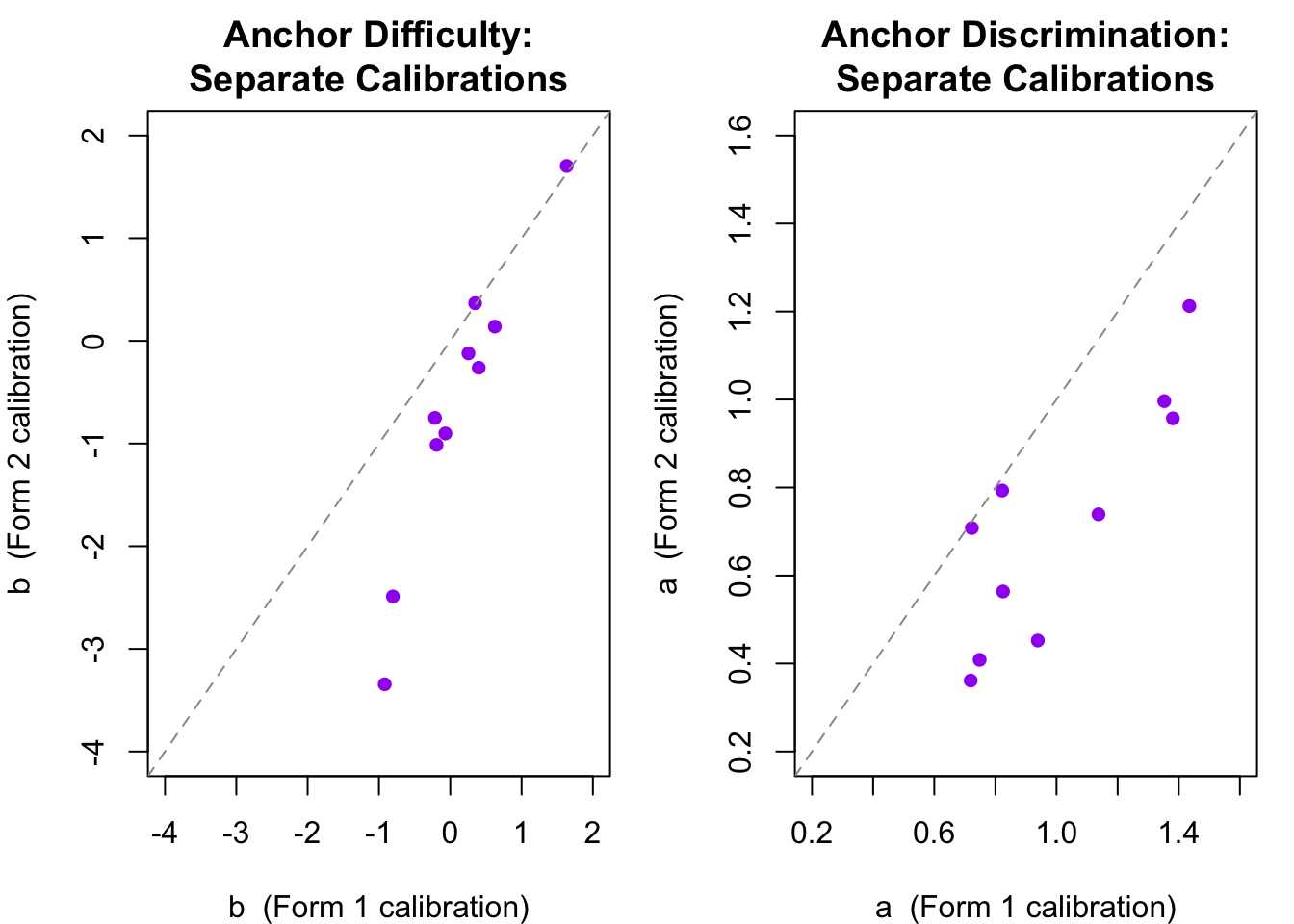
What happened? When `mirt` estimates item parameters it anchors the logit scale by fixing the mean and SD of the population distribution to 0 and 1. This is the actual mean and SD for the Group 1 sample---but it is **not** the mean and SD we generated for Group 2. The two sets of thetas appear to be on the same scale, but they are not. Let's see this by comparing the estimated difficulty and discrimination parameters for the 10 anchor items.
```{r anchor-param-comparison}
par(mfrow = c(1, 2), mar = c(4, 4, 3, 1))

# Anchor item difficulties
plot(items1[1:10, 2], items2[1:10, 2],
     xlab = "b  (Form 1 calibration)", ylab = "b  (Form 2 calibration)",
     main = "Anchor Difficulty:\nSeparate Calibrations",
     pch = 16, col = "purple", xlim = c(-4, 2), ylim = c(-4, 2))
abline(a = 0, b = 1, lty = 2, col = "gray60")

# Anchor item discriminations
plot(items1[1:10, 1], items2[1:10, 1],
     xlab = "a  (Form 1 calibration)", ylab = "a  (Form 2 calibration)",
     main = "Anchor Discrimination:\nSeparate Calibrations",
     pch = 16, col = "purple", xlim = c(.2, 1.6), ylim = c(.2, 1.6))
abline(a = 0, b = 1, lty = 2, col = "gray60")
par(mfrow = c(1, 1))
```
The two sets of estimates are strongly correlated---supporting parameter invariance---but systematically offset from the identity line. They are not on the same scale. The pattern here (a systematic shift rather than random scatter) is exactly what the IRT linking transformation is designed to correct.
---
## Equating with Separate Calibration and Linking Constants
Having confirmed the scale mismatch, we can now estimate the **linking constants** $A$ and $B$ that map the Form 2 scale onto the Form 1 scale. Recall from the background reading that if we define $\theta_1 = A \cdot \theta_2 + B$, then the anchor item parameters must satisfy:
$$b_1 = A \cdot b_2 + B \qquad \text{and} \qquad a_1 = \frac{a_2}{A}$$
In the separate IRT equating approach we can estimate $A$ and $B$ from the 10 anchor items using three different methods.
### Mean-Mean Method
The **mean-mean** method estimates $A$ from the ratio of mean discrimination parameters across the two calibrations, and $B$ from the adjusted mean difference in difficulty parameters.
```{r mean-mean}
# Anchor item parameters from each separate calibration (items 1-10)
a1_anc <- items1[1:10, 1];  b1_anc <- items1[1:10, 2]
a2_anc <- items2[1:10, 1];  b2_anc <- items2[1:10, 2]

A_mm <- mean(a2_anc) / mean(a1_anc)
B_mm <- mean(b1_anc) - A_mm * mean(b2_anc)

cat("Mean-Mean:  A =", round(A_mm, 4), "  B =", round(B_mm, 4), "\n")
```
### Mean-Sigma Method
The **mean-sigma** method estimates $A$ from the ratio of the standard deviations of the anchor *difficulty* parameters (which are typically estimated more stably than discriminations), and $B$ from the mean difference in difficulties.
```{r mean-sigma}
A_ms <- sd(b1_anc) / sd(b2_anc)
B_ms <- mean(b1_anc) - A_ms * mean(b2_anc)

cat("Mean-Sigma: A =", round(A_ms, 4), "  B =", round(B_ms, 4), "\n")
```
We expect $A < 1$ and $B > 0$ here. Recall that Group 2 has higher mean ability ($\mu = 0.5$) but less variability ($\sigma = 0.8$) than Group 1 ($\mu = 0$, $\sigma = 1$). When `mirt` separately calibrates Form 2, it forces the $N(0.5, 0.8)$ ability distribution onto a $N(0, 1)$ scale. This has two consequences. First, the $\theta$ scale gets *stretched*---the true SD of 0.8 is expanded to 1---which inflates the spread of the $b$-parameter estimates and compresses the $a$-parameter estimates. Second, the origin gets *shifted* downward---the true mean of 0.5 is pulled to 0. The linking constant $A < 1$ undoes the stretching, scaling Form 2's parameters back to the narrower Form 1 metric, while $B > 0$ undoes the shift, moving the zero-centered Form 2 scale upward to reflect Group 2's higher mean. Notice, however, that the Mean-Mean and Mean-Sigma methods give noticeably different estimates of $A$. This discrepancy is a warning sign that moment-based summaries of the anchor item parameters can be unstable.
### Stocking-Lord Method
The **Stocking-Lord** method (Stocking & Lord, 1983) takes a different approach. Rather than summarizing the anchor parameters with means or standard deviations, it finds the $A$ and $B$ that minimize the squared difference between the anchor **test characteristic curves** (TCCs) evaluated on the two scales. In notation from Kolen and Brennan (2014, Eq. 6.15), the criterion is:
$$SL_{\text{crit}} = \sum_{k} \left[ \sum_{j \in V} p_j\!\left(\theta_k;\, \hat{a}_{1j},\, \hat{b}_{1j}\right) \;-\; \sum_{j \in V} p_j\!\left(\theta_k;\, \frac{\hat{a}_{2j}}{A},\, A\hat{b}_{2j} + B\right) \right]^2$$
where $V$ denotes the set of anchor items and $\theta_k$ ranges over a grid of ability values. The key advantage is that this criterion considers all item parameters simultaneously, so a single item with an extreme $\hat{b}$ or $\hat{a}$ estimate cannot dominate the way it can with moment-based methods. We implement this directly with `optim`, using the mean-mean constants as starting values.
```{r stocking-lord}
# 2PL item characteristic curve
icc_2pl <- function(theta, a, b) 1 / (1 + exp(-a * (theta - b)))

# Test characteristic curve: sum of ICCs across items at each theta point
tcc_2pl <- function(theta, a, b) {
  sapply(theta, function(th) sum(icc_2pl(th, a, b)))
}

# Stocking-Lord criterion function
stocking_lord <- function(a1, b1, a2, b2,
                          theta = seq(-4, 4, by = 0.1),
                          start_A = NULL, start_B = NULL) {
  # Compute target TCC once (Form 1 anchor items)
  tcc_target <- tcc_2pl(theta, a1, b1)

  # Criterion: sum of squared TCC differences
  sl_criterion <- function(par) {
    A <- par[1]; B <- par[2]
    tcc_source <- tcc_2pl(theta, a2 / A, A * b2 + B)
    sum((tcc_target - tcc_source)^2)
  }

  # Starting values from mean-mean if not supplied
  if (is.null(start_A)) start_A <- mean(a2) / mean(a1)
  if (is.null(start_B)) start_B <- mean(b1) - start_A * mean(b2)

  result <- optim(c(start_A, start_B), sl_criterion, method = "Nelder-Mead")
  list(A = result$par[1], B = result$par[2],
       convergence = result$convergence, criterion = result$value)
}

sl <- stocking_lord(a1_anc, b1_anc, a2_anc, b2_anc)
cat("Stocking-Lord: A =", round(sl$A, 4), "  B =", round(sl$B, 4), "\n")
```
The Stocking-Lord $A$ and $B$ fall between the mean-mean and mean-sigma estimates. Because the optimization considers the full shape of each anchor item's characteristic curve, it is less sensitive to any single extreme parameter estimate.
### Applying the Transformation
We apply the linking constants to transform Form 2 item parameters onto the Form 1 scale.
```{r apply-transform}
# Extract Stocking-Lord constants
A_sl <- sl$A;  B_sl <- sl$B

# Transform Form 2 item parameters to Form 1 scale using each method
b2_mm <- A_mm * items2[, 2] + B_mm;  a2_mm <- items2[, 1] / A_mm
b2_ms <- A_ms * items2[, 2] + B_ms;  a2_ms <- items2[, 1] / A_ms
b2_sl <- A_sl * items2[, 2] + B_sl;  a2_sl <- items2[, 1] / A_sl

# Compare implied Group 2 population parameters to true generating values.
# On Form 2's mirt scale the population is N(0, 1) by construction.
# After the linear transformation theta_1 = A * theta_2 + B, the implied
# population mean = A * 0 + B = B and the implied population SD = A * 1 = A.
comp_sep <- data.frame(
  Version = c("Form 2 -- no transformation",
              "Form 2 -- Mean-Mean",
              "Form 2 -- Mean-Sigma",
              "Form 2 -- Stocking-Lord",
              "True generating value"),
  Mean_th = c(0.000, round(B_mm, 3), round(B_ms, 3), round(B_sl, 3), 0.500),
  SD_th   = c(1.000, round(A_mm, 3), round(A_ms, 3), round(A_sl, 3), 0.800)
)

comp_sep |>
  kable("html", col.names = c("Version", "Mean (θ)", "SD (θ)")) |>
  kable_styling(full_width = FALSE)
```
Without transformation, `mirt`'s identification constraint forces the Form 2 population to N(0, 1), masking the true group difference. After applying the linking constants, the implied population mean on the Form 1 scale is $B$ and the implied population SD is $A$.
The Stocking-Lord method recovers the population mean most accurately among the three separate calibration approaches. All three underestimate the population SD, but the mean-sigma method is the worst offender---its $A$ depends on the ratio of standard deviations of the anchor difficulty estimates, and on the Form 2 scale a few easy anchor items have extreme $\hat{b}$ values that inflate $\text{sd}(\hat{b}_2)$, pulling $A$ too low. The mean-mean and Stocking-Lord methods are less sensitive to these outliers, though neither fully recovers the true SD in this instance. This general pattern---moment-based methods being less stable than characteristic curve methods---is well documented (Kolen & Brennan, 2014, Section 6.3.4).
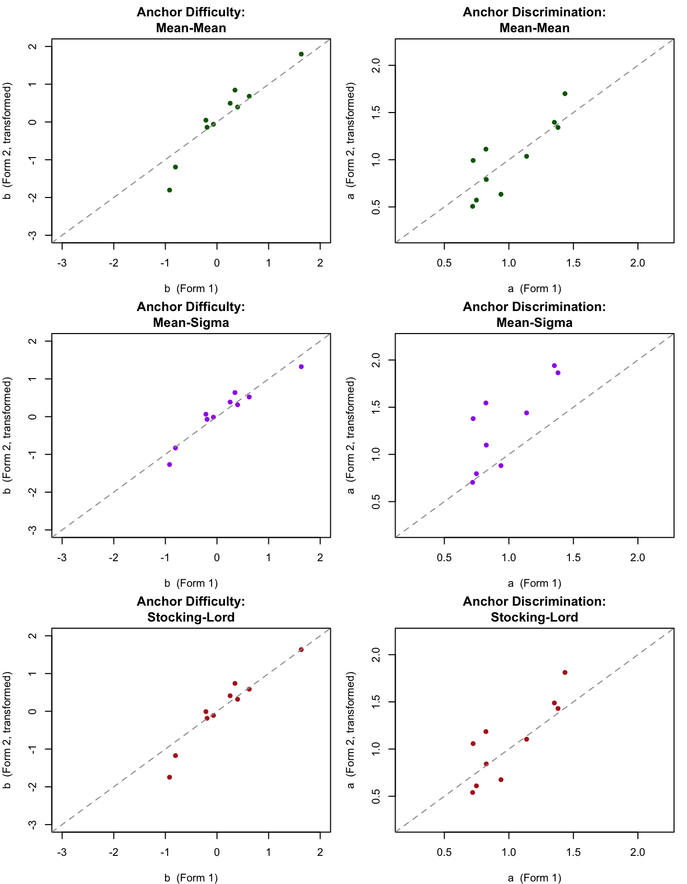
Let's check how well the anchor item parameters align after each transformation.
```{r sep-anchor-check, fig.height=9}
par(mfrow = c(3, 2), mar = c(4, 4, 3, 1))

# Mean-Mean
plot(items1[1:10, 2], b2_mm[1:10],
     xlab = "b  (Form 1)", ylab = "b  (Form 2, transformed)",
     main = "Anchor Difficulty:\nMean-Mean",
     pch = 16, col = "darkgreen", xlim = c(-3, 2), ylim = c(-3, 2))
abline(a = 0, b = 1, lty = 2, col = "gray60")

plot(items1[1:10, 1], a2_mm[1:10],
     xlab = "a  (Form 1)", ylab = "a  (Form 2, transformed)",
     main = "Anchor Discrimination:\nMean-Mean",
     pch = 16, col = "darkgreen", xlim = c(0.2, 2.2), ylim = c(0.2, 2.2))
abline(a = 0, b = 1, lty = 2, col = "gray60")

# Mean-Sigma
plot(items1[1:10, 2], b2_ms[1:10],
     xlab = "b  (Form 1)", ylab = "b  (Form 2, transformed)",
     main = "Anchor Difficulty:\nMean-Sigma",
     pch = 16, col = "purple", xlim = c(-3, 2), ylim = c(-3, 2))
abline(a = 0, b = 1, lty = 2, col = "gray60")

plot(items1[1:10, 1], a2_ms[1:10],
     xlab = "a  (Form 1)", ylab = "a  (Form 2, transformed)",
     main = "Anchor Discrimination:\nMean-Sigma",
     pch = 16, col = "purple", xlim = c(0.2, 2.2), ylim = c(0.2, 2.2))
abline(a = 0, b = 1, lty = 2, col = "gray60")

# Stocking-Lord
plot(items1[1:10, 2], b2_sl[1:10],
     xlab = "b  (Form 1)", ylab = "b  (Form 2, transformed)",
     main = "Anchor Difficulty:\nStocking-Lord",
     pch = 16, col = "firebrick", xlim = c(-3, 2), ylim = c(-3, 2))
abline(a = 0, b = 1, lty = 2, col = "gray60")

plot(items1[1:10, 1], a2_sl[1:10],
     xlab = "a  (Form 1)", ylab = "a  (Form 2, transformed)",
     main = "Anchor Discrimination:\nStocking-Lord",
     pch = 16, col = "firebrick", xlim = c(0.2, 2.2), ylim = c(0.2, 2.2))
abline(a = 0, b = 1, lty = 2, col = "gray60")
par(mfrow = c(1, 1))
```
The mean-mean transformation (top row) and Stocking-Lord transformation (bottom row) both bring the anchor parameters reasonably close to the identity line. The mean-sigma difficulty plot (middle left) shows the transformed parameters compressed toward 0---a consequence of the underestimated $A$ constant. Items that deviate substantially from the identity line after any transformation may be showing differential item functioning across the two groups. When the groups are defined by time (e.g. 2024 vs 2025), this is known as "item parameter drift."
### On Your Own
1. Try transforming the Form 2 *unique* item parameters (items 11--20) using the Stocking-Lord constants and compare them to the true generating values (`b2[11:20]` and `a2[11:20]`). How well did the linking recover the truth?
2. The mean-sigma method ignores discrimination parameters when estimating $A$. Based on the results here, why is that a problem?
---
## Equating with Anchored Calibration
Let's try the second of the three IRT equating approaches. We re-calibrate the items for Form 2, but this time we anchor the first 10 items to have the same difficulty and discrimination values estimated for Form 1.
```{r anchored-calibration}
# Discrimination parameters for anchor items (Form 1 estimates)
anchor_a <- items1[1:10, 1]
# Difficulty parameters converted to mirt's slope-intercept "d" parameterization
anchor_d <- -anchor_a * items1[1:10, 2]

# Get starting values for Form 2 calibration
sv2 <- mirt(test2, 1, itemtype = '2PL', pars = 'values', verbose = FALSE)

# Fix anchor item slope and intercept parameters (parnum < 41 covers items 1-10)
sv2$value[sv2$name == 'a1' & sv2$parnum < 41] <- anchor_a
sv2$value[sv2$name == 'd'  & sv2$parnum < 41] <- anchor_d
sv2$est[sv2$parnum < 41] <- FALSE

# Free the population mean and variance so they can be estimated
sv2$est[sv2$name == 'MEAN_1'] <- TRUE
sv2$est[sv2$name == 'COV_11'] <- TRUE

# Fit the 2PL with anchor constraints
fit2.a    <- mirt(test2, 1, pars = sv2, verbose = FALSE)
items2.a  <- coef(fit2.a, IRTpars = TRUE, simplify = TRUE)$items
coef(fit2.a, IRTpars = TRUE, simplify = TRUE)
```
Now let's compare the mean and SD of the two theta distributions after anchoring the Form 2 scale to Form 1.
```{r pop-comparison-anchored}
comp_anc <- data.frame(
  Form = c("Form 1 (Group 1)", "Form 2 Anchored (Group 2)"),
  Mean = c(coef(fit1)$GroupPars[1],  coef(fit2.a)$GroupPars[1]),
  SD   = c(sqrt(coef(fit1)$GroupPars[2]), sqrt(coef(fit2.a)$GroupPars[2]))
)
comp_anc |>
  kable("html", digits = 3, col.names = c("Form", "Mean (θ)", "SD (θ)")) |>
  kable_styling(full_width = FALSE)
```
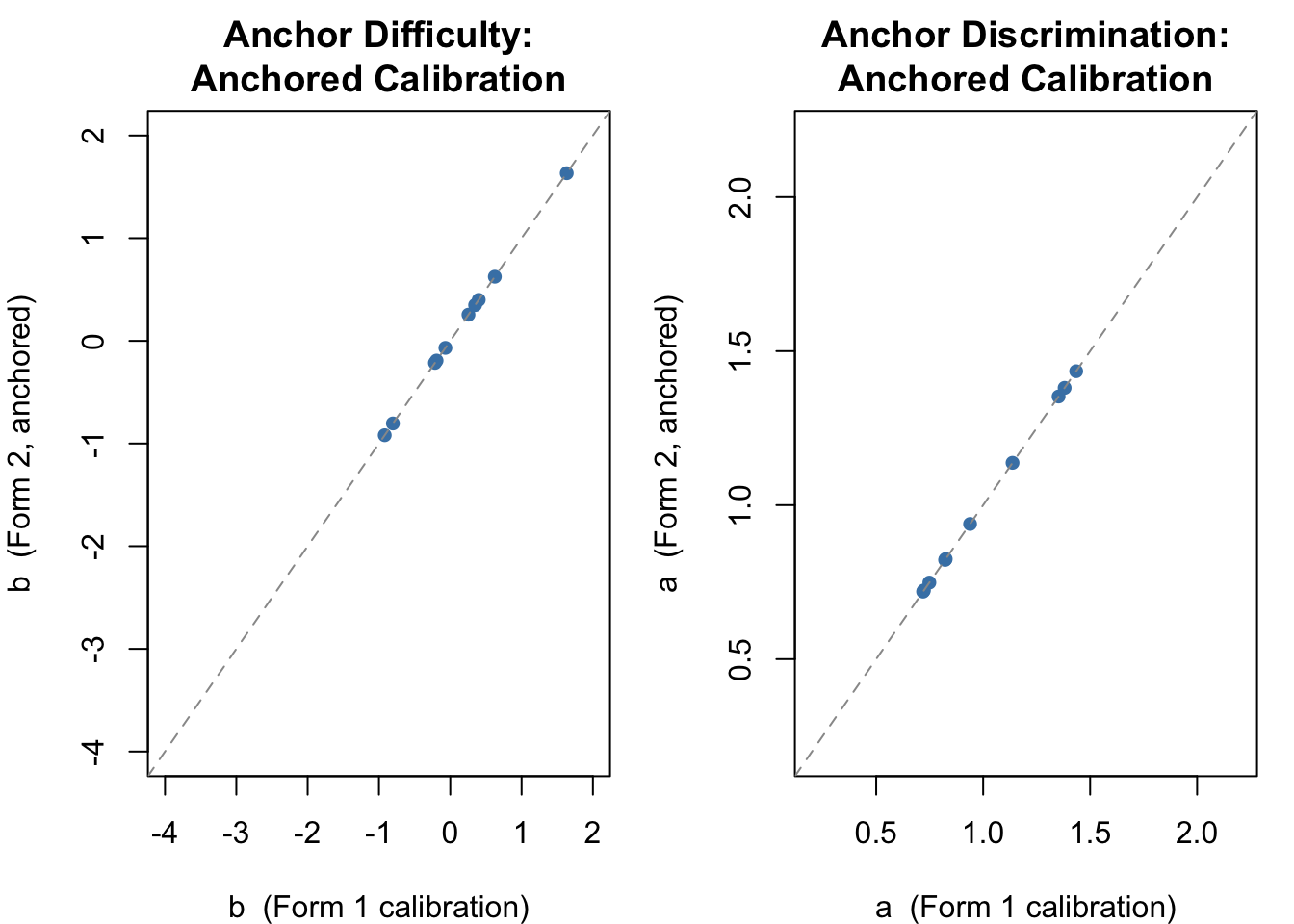
We are now close to the true generating values for Group 2 ($\mu = 0.5$, $\sigma = 0.8$). We can also verify that the item parameter estimates for the 10 anchor items are identical across the two calibrations---we forced this to be so.
```{r anchor-check-anchored}
par(mfrow = c(1, 2), mar = c(4, 4, 3, 1))

# Anchor difficulties
plot(items1[1:10, 2], items2.a[1:10, 2],
     xlab = "b  (Form 1 calibration)", ylab = "b  (Form 2, anchored)",
     main = "Anchor Difficulty:\nAnchored Calibration",
     pch = 16, col = "steelblue", xlim = c(-4, 2), ylim = c(-4, 2))
abline(a = 0, b = 1, lty = 2, col = "gray60")

# Anchor discriminations
plot(items1[1:10, 1], items2.a[1:10, 1],
     xlab = "a  (Form 1 calibration)", ylab = "a  (Form 2, anchored)",
     main = "Anchor Discrimination:\nAnchored Calibration",
     pch = 16, col = "steelblue", xlim = c(.2, 2.2), ylim = c(.2, 2.2))
abline(a = 0, b = 1, lty = 2, col = "gray60")
par(mfrow = c(1, 1))
```
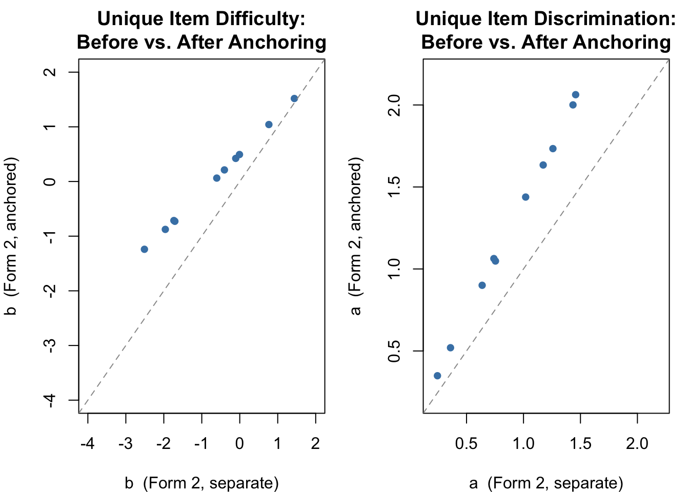
The more interesting comparison is of the unique items (11--20) on Form 2, before and after anchoring.
```{r unique-check-anchored}
par(mfrow = c(1, 2), mar = c(4, 4, 3, 1))

# Unique item difficulties
plot(items2[11:20, 2], items2.a[11:20, 2],
     xlab = "b  (Form 2, separate)", ylab = "b  (Form 2, anchored)",
     main = "Unique Item Difficulty:\nBefore vs. After Anchoring",
     pch = 16, col = "steelblue", xlim = c(-4, 2), ylim = c(-4, 2))
abline(a = 0, b = 1, lty = 2, col = "gray60")

# Unique item discriminations
plot(items2[11:20, 1], items2.a[11:20, 1],
     xlab = "a  (Form 2, separate)", ylab = "a  (Form 2, anchored)",
     main = "Unique Item Discrimination:\nBefore vs. After Anchoring",
     pch = 16, col = "steelblue", xlim = c(.2, 2.2), ylim = c(.2, 2.2))
abline(a = 0, b = 1, lty = 2, col = "gray60")
par(mfrow = c(1, 1))
```
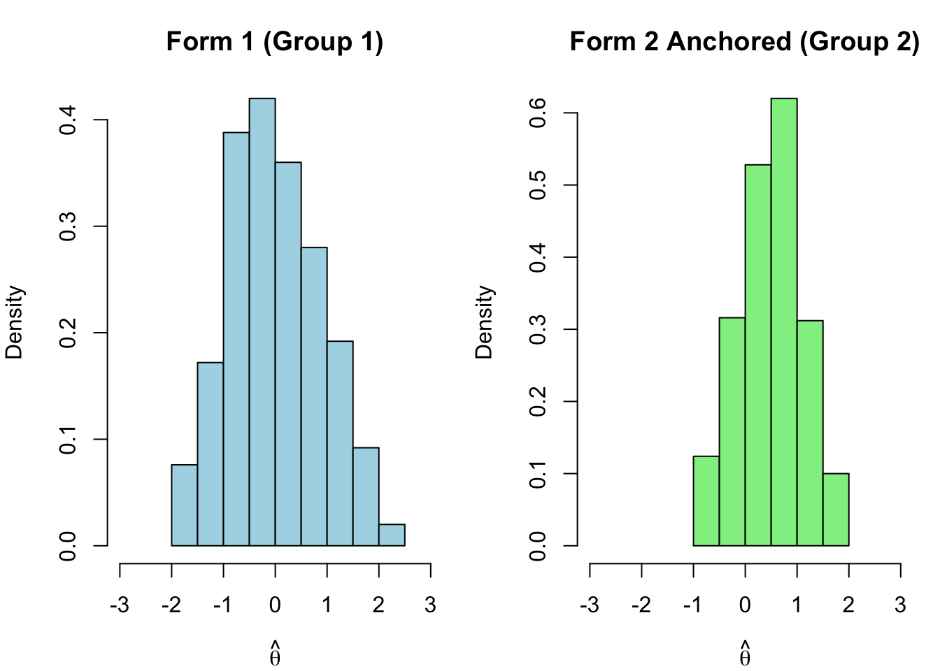
With both forms now on the same scale, we can obtain EAP theta estimates from each and compare them directly.
```{r theta-comparison-anchored}
th1.eap   <- fscores(fit1)[, 1]
th2.a.eap <- fscores(fit2.a)[, 1]

par(mfrow = c(1, 2), mar = c(4, 4, 3, 1))
hist(th1.eap,   xlim = c(-3, 3), main = "Form 1 (Group 1)",
     xlab = expression(hat(theta)), col = "lightblue",  freq = FALSE)
hist(th2.a.eap, xlim = c(-3, 3), main = "Form 2 Anchored (Group 2)",
     xlab = expression(hat(theta)), col = "lightgreen", freq = FALSE)
par(mfrow = c(1, 1))
```
### On Your Own
1. Compare the estimated item parameters to their generating values---how did we do?
2. Should we be concerned that we are underestimating the true SD of the theta distribution for Group 2?
3. Would we do better if we had more students? More anchor items? Better-discriminating anchor items?
---
## Concurrent Calibration
The first thing we need to do is restructure the data from the two forms into a single dataframe.
```{r concurrent-data}
# We reuse the test1 and test2 matrices simulated at the top of this document.
# (Re-simulating here without resetting the seed would produce different data.)

# Rename the last 10 columns of test2 to distinguish them from Form 1 unique items
new_labels <- paste0("Item_", (ncol(test2) + 1):(ncol(test2) + 10))
colnames(test2)[(ncol(test2) - 9):ncol(test2)] <- new_labels

# Group membership vector (used by multipleGroup)
group <- c(rep("Test1", 500), rep("Test2", 500))

# Add group indicator column for merging
test1 <- mutate(test1, group = 1)
test2 <- mutate(test2, group = 2)

# Merge on common anchor items (Item_1 through Item_10)
common_items <- paste0("Item_", 1:10)
full_dat <- merge(test1, test2, by = c("group", common_items),
                  all.x = TRUE, all.y = TRUE)
dat <- full_dat[, -1]
```
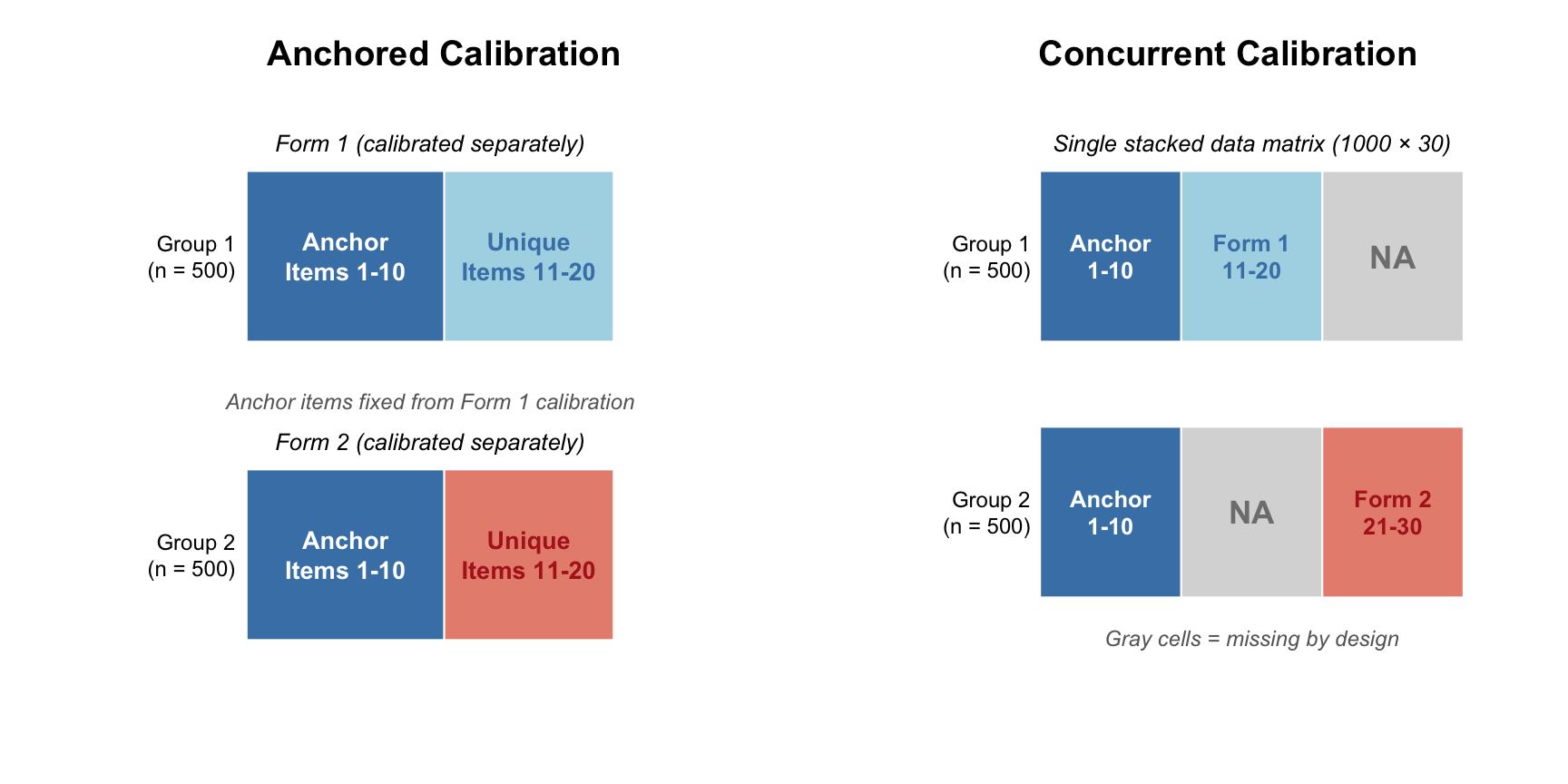
Notice the structure of `full_dat`. For the first 500 cases (students taking Form 1), we have observations for items 1--20; items 21--30 are missing by design. For the next 500 cases (students taking Form 2), we have observations for items 1--10 (the anchor items) and items 21--30 (Form 2 unique items); items 11--20 are missing by design. The diagram below contrasts this stacked data layout with the separate-forms layout used in the anchored calibration.
```{r data-structure-diagram, echo=FALSE, fig.height=4.5, fig.width=9}
par(mfrow = c(1, 2), mar = c(1, 4, 3, 1))
# --- Left panel: Anchored calibration (separate forms) ---
plot(NULL, xlim = c(0, 10), ylim = c(0, 7), axes = FALSE,
xlab = "", ylab = "", main = "Anchored Calibration")
# Form 1 block
rect(1.5, 4.5, 5, 6.5, col = "steelblue", border = "white")
rect(5, 4.5, 8, 6.5, col = "lightblue", border = "white")
text(3.25, 5.5, "Anchor\nItems 1-10", cex = 0.85, font = 2, col = "white")
text(6.5, 5.5, "Unique\nItems 11-20", cex = 0.85, font = 2, col = "steelblue")
# Form 2 block
rect(1.5, 1, 5, 3, col = "steelblue", border = "white")
rect(5, 1, 8, 3, col = "#E8907E", border = "white")
text(3.25, 2, "Anchor\nItems 1-10", cex = 0.85, font = 2, col = "white")
text(6.5, 2, "Unique\nItems 11-20", cex = 0.85, font = 2, col = "firebrick")
# Row labels
text(1.3, 5.5, "Group 1\n(n = 500)", cex = 0.75, adj = 1)
text(1.3, 2, "Group 2\n(n = 500)", cex = 0.75, adj = 1)
# Annotations
text(4.75, 6.8, "Form 1 (calibrated separately)", cex = 0.8, font = 3)
text(4.75, 3.3, "Form 2 (calibrated separately)", cex = 0.8, font = 3)
text(4.75, 3.8, "Anchor items fixed from Form 1 calibration",
cex = 0.75, font = 3, col = "gray40")
# --- Right panel: Concurrent calibration (stacked) ---
plot(NULL, xlim = c(0, 12), ylim = c(0, 7), axes = FALSE,
xlab = "", ylab = "", main = "Concurrent Calibration")
# Group 1 row: anchor + Form 1 unique (observed), Form 2 unique (missing)
rect(2, 4.5, 5, 6.5, col = "steelblue", border = "white")
rect(5, 4.5, 8, 6.5, col = "lightblue", border = "white")
rect(8, 4.5, 11, 6.5, col = "gray85", border = "white")
text(3.5, 5.5, "Anchor\n1-10", cex = 0.8, font = 2, col = "white")
text(6.5, 5.5, "Form 1\n11-20", cex = 0.8, font = 2, col = "steelblue")
text(9.5, 5.5, "NA", cex = 1.1, font = 2, col = "gray50")
# Group 2 row: anchor (observed), Form 1 unique (missing), Form 2 unique (observed)
rect(2, 1.5, 5, 3.5, col = "steelblue", border = "white")
rect(5, 1.5, 8, 3.5, col = "gray85", border = "white")
rect(8, 1.5, 11, 3.5, col = "#E8907E", border = "white")
text(3.5, 2.5, "Anchor\n1-10", cex = 0.8, font = 2, col = "white")
text(6.5, 2.5, "NA", cex = 1.1, font = 2, col = "gray50")
text(9.5, 2.5, "Form 2\n21-30", cex = 0.8, font = 2, col = "firebrick")
# Row labels
text(1.8, 5.5, "Group 1\n(n = 500)", cex = 0.75, adj = 1)
text(1.8, 2.5, "Group 2\n(n = 500)", cex = 0.75, adj = 1)
# Annotation
text(6.5, 6.8, "Single stacked data matrix (1000 × 30)", cex = 0.8, font = 3)
text(6.5, 1, expression(italic("Gray cells = missing by design")), cex = 0.75, col = "gray40")
par(mfrow = c(1, 1))
```
Now we are ready to do a concurrent multigroup calibration using `mirt`.
```{r concurrent-calibration}
cc <- multipleGroup(dat, model = 1, group = group, itemtype = '2PL',
                    invariance = c('intercepts', 'slopes', 'free_var', 'free_means'),
                    verbose = FALSE)

out.cc <- coef(cc, simplify = TRUE, IRTpars = TRUE)
out.cc
# To access directly:
# out.cc$Test1$items  -- item parameters for Form 1 reference group
# out.cc$Test2$items  -- item parameters for Form 2 focus group
```
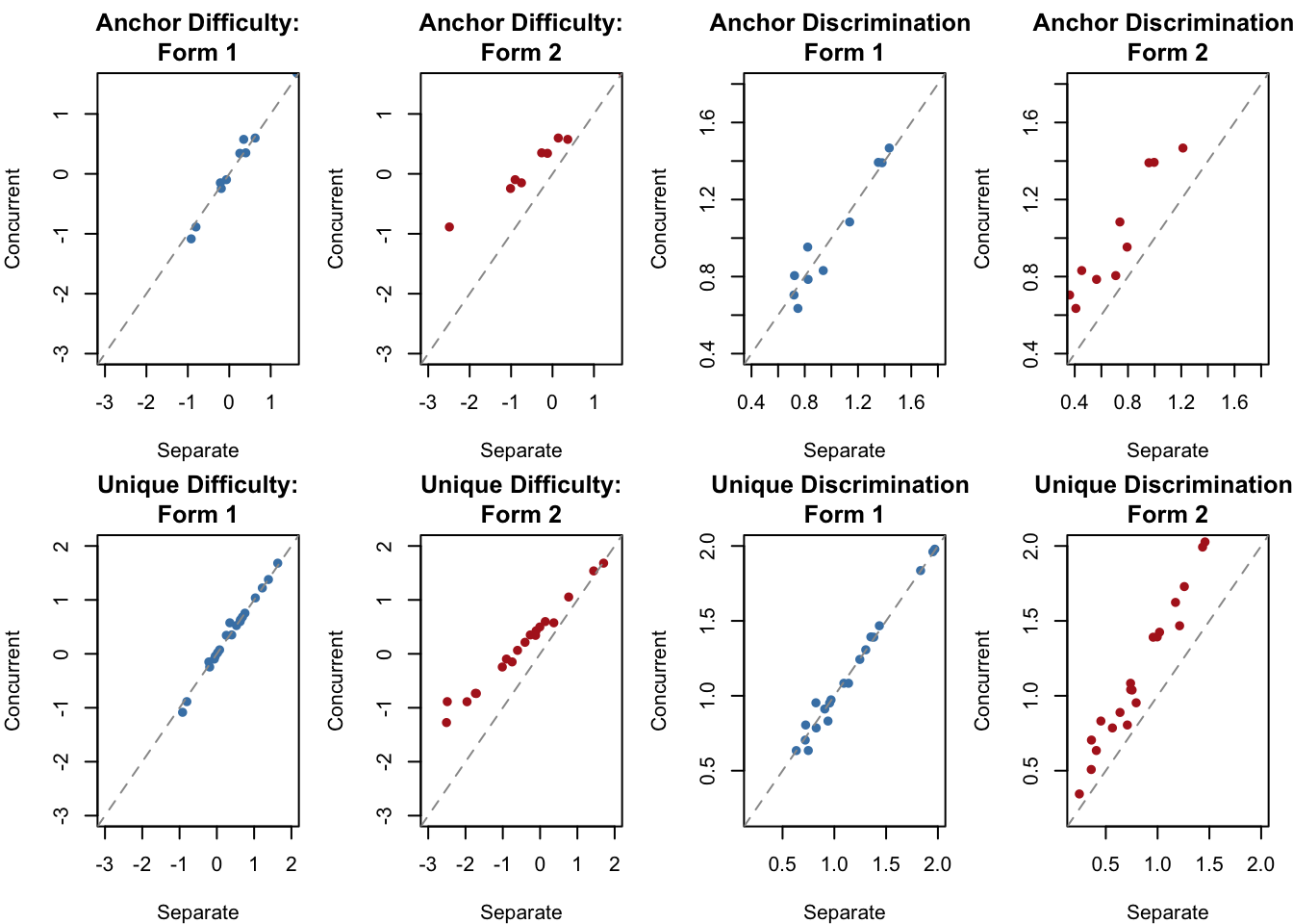
In the multigroup concurrent calibration, the mean and variance of the reference group (Test1) are fixed at 0 and 1, while those of the focus group are freely estimated. You can access them via `out.cc$Test2$means` (population mean) and `out.cc$Test2$cov` (population variance). Let's compare the item parameters from the concurrent calibration to those from the two separate calibrations.
```{r concurrent-comparison-plots}
par(mfrow = c(2, 4), mar = c(4, 4, 3, 1))

# Common item difficulty -- Form 1 separate vs. concurrent
plot(items1[1:10, 2], out.cc$Test1$items[1:10, 2],
     xlab = "Separate", ylab = "Concurrent",
     main = "Anchor Difficulty:\nForm 1",
     pch = 16, col = "steelblue", xlim = c(-3, 1.5), ylim = c(-3, 1.5))
abline(a = 0, b = 1, lty = 2, col = "gray60")

# Common item difficulty -- Form 2 separate vs. concurrent
plot(items2[1:10, 2], out.cc$Test1$items[1:10, 2],
     xlab = "Separate", ylab = "Concurrent",
     main = "Anchor Difficulty:\nForm 2",
     pch = 16, col = "firebrick", xlim = c(-3, 1.5), ylim = c(-3, 1.5))
abline(a = 0, b = 1, lty = 2, col = "gray60")

# Common item discrimination -- Form 1 separate vs. concurrent
plot(items1[1:10, 1], out.cc$Test1$items[1:10, 1],
     xlab = "Separate", ylab = "Concurrent",
     main = "Anchor Discrimination:\nForm 1",
     pch = 16, col = "steelblue", xlim = c(.4, 1.8), ylim = c(.4, 1.8))
abline(a = 0, b = 1, lty = 2, col = "gray60")

# Common item discrimination -- Form 2 separate vs. concurrent
plot(items2[1:10, 1], out.cc$Test1$items[1:10, 1],
     xlab = "Separate", ylab = "Concurrent",
     main = "Anchor Discrimination:\nForm 2",
     pch = 16, col = "firebrick", xlim = c(.4, 1.8), ylim = c(.4, 1.8))
abline(a = 0, b = 1, lty = 2, col = "gray60")

# Unique item difficulty -- Form 1
plot(items1[, 2], out.cc$Test1$items[1:20, 2],
     xlab = "Separate", ylab = "Concurrent",
     main = "Unique Difficulty:\nForm 1",
     pch = 16, col = "steelblue", xlim = c(-3, 2), ylim = c(-3, 2))
abline(a = 0, b = 1, lty = 2, col = "gray60")

# Unique item difficulty -- Form 2
plot(items2[, 2], out.cc$Test2$items[c(1:10, 21:30), 2],
     xlab = "Separate", ylab = "Concurrent",
     main = "Unique Difficulty:\nForm 2",
     pch = 16, col = "firebrick", xlim = c(-3, 2), ylim = c(-3, 2))
abline(a = 0, b = 1, lty = 2, col = "gray60")

# Unique item discrimination -- Form 1
plot(items1[, 1], out.cc$Test1$items[1:20, 1],
     xlab = "Separate", ylab = "Concurrent",
     main = "Unique Discrimination:\nForm 1",
     pch = 16, col = "steelblue", xlim = c(.2, 2), ylim = c(.2, 2))
abline(a = 0, b = 1, lty = 2, col = "gray60")

# Unique item discrimination -- Form 2
plot(items2[, 1], out.cc$Test2$items[c(1:10, 21:30), 1],
     xlab = "Separate", ylab = "Concurrent",
     main = "Unique Discrimination:\nForm 2",
     pch = 16, col = "firebrick", xlim = c(.2, 2), ylim = c(.2, 2))
abline(a = 0, b = 1, lty = 2, col = "gray60")
par(mfrow = c(1, 1))
```
The concurrent calibration places all 30 items on a single common scale in one step. Form 1 item parameters (blue) are estimated from data on the reference scale and so fall close to the identity line. Form 2 item parameters (red) come from a separate scale in the independent calibrations but are brought onto the Form 1 scale in the concurrent calibration, producing a systematic shift relative to the identity line.
---
## Comparing All Approaches
We have now implemented separate calibration (with three different methods for estimating linking constants), anchored calibration, and concurrent calibration. Let's compare the key result from each: the estimated mean and standard deviation of the Group 2 ability distribution on the Form 1 scale, compared to the true generating values ($\mu = 0.5$, $\sigma = 0.8$).
```{r comparison}
# Population estimates from concurrent calibration
cc_mean <- out.cc$Test2$means[1]
cc_sd   <- sqrt(out.cc$Test2$cov[1])

# Population estimates from anchored calibration
anc_mean <- coef(fit2.a)$GroupPars[1]
anc_sd   <- sqrt(coef(fit2.a)$GroupPars[2])

# For separate calibration, the implied population mean = B and SD = A
# (because the Form 2 population is N(0,1) by mirt's identification constraint)
comparison <- data.frame(
  Method = c("True (generating)",
             "Separate + Mean-Mean",
             "Separate + Mean-Sigma",
             "Separate + Stocking-Lord",
             "Anchored",
             "Concurrent"),
  Group2_Mean = c(0.500,
                  round(B_mm,     3),
                  round(B_ms,     3),
                  round(B_sl,     3),
                  round(anc_mean, 3),
                  round(cc_mean,  3)),
  Group2_SD   = c(0.800,
                  round(A_mm,     3),
                  round(A_ms,     3),
                  round(A_sl,     3),
                  round(anc_sd,   3),
                  round(cc_sd,    3))
)

comparison |>
  kable("html", col.names = c("Method", "Group 2 Mean (θ)", "Group 2 SD (θ)")) |>
  kable_styling(full_width = FALSE)
```
Several patterns stand out. For recovering the Group 2 mean, the Stocking-Lord, anchored, and concurrent approaches are all very close to the true value; the moment-based methods (mean-mean, mean-sigma) are less accurate. For the SD, all methods underestimate the true value of 0.8 to some degree. The anchored, concurrent, and mean-mean methods cluster together, the Stocking-Lord method is somewhat lower, and the mean-sigma method is clearly the worst. The mean-sigma $A$ is dragged too low by a few anchor items with extreme $\hat{b}$ values on the Form 2 scale.
In practice, Kolen and Brennan (2014, Section 6.3.4) recommend using the Stocking-Lord or Haebara characteristic curve methods when separate calibration is used, primarily because they are more **stable across replications** than the moment-based methods, even if any single realization may not show dramatic differences. When feasible, anchored or concurrent calibration avoids the linking constant estimation problem entirely.
---
## On Your Own
1. Does the overall flow of results across the approaches make sense to you? Give it some thought.
2. Compare the estimated item parameters from each approach to the true generating values (`b1`, `b2`, `a1`, `a2`). Which approach recovers the truth most accurately for the unique items?
3. All methods underestimate the true SD (0.8) of the Group 2 theta distribution to some degree. What might cause this?
4. Look at the anchor item $b$-parameter estimates on the two scales. Which items have the most extreme Form 2 estimates? Why might that be, and how does it affect the mean-sigma linking constant?
5. Try running the simulation with different seeds (e.g., `set.seed(42)`, `set.seed(100)`). How stable are the linking constants across replications? Which method shows the most variability?
6. The anchor test here is 10 out of 20 items (50% of the test). What would you expect to happen to equating accuracy if the anchor were only 5 items? Try modifying the simulation to find out.