13  Evaluating IRT Model Fit

14 Introduction

Fitting an IRT model to data is just the beginning. Before drawing any substantive conclusions from the model—whether about item quality, examinee proficiency, or test characteristics—we need to evaluate how well the model actually fits the data. A model that doesn’t fit is, at best, a rough approximation, and at worst, a source of misleading inferences.

Why does model fit matter? IRT models make strong assumptions:

• Unidimensionality: A single latent trait \(\theta\) underlies responses to all items.
• Local independence: Conditional on \(\theta\), item responses are statistically independent.
• Correct functional form: The ICC (Item Characteristic Curve) accurately describes the probability of a correct response as a function of \(\theta\).

When these assumptions are violated, parameter estimates can be biased, standard errors can be inaccurate, and the model-based inferences we care about can break down.

Levels of fit evaluation. We will examine fit at multiple levels:

1. Overall model comparison – Which model (1PL, 2PL, 3PL) best balances fit and parsimony?
2. Item-level fit – Do individual items conform to the model? Which items are problematic?
3. Person-level fit – Are there examinees whose response patterns are inconsistent with the model?
4. Assumption checks – Is there evidence against unidimensionality or local independence?

Packages. We will use mirt (Chalmers, 2012) for IRT modeling and fit evaluation, CTT for classical item analysis, and psych for parallel analysis.

library(CTT)
library(mirt)
library(psych)
library(knitr)
library(kableExtra)

Data. Our example data set is a subsample of \(N = 1{,}500\) examinees from the Colorado Department of Education (CDE) math assessment, consisting of 31 dichotomously scored items.

d <- read.csv(file = "~/Dropbox/Courses/EDUC 8720/Data Sets/MASC-CDE/cde_subsample_math.csv")
dim(d)

#> [1] 1500   31

15 Classical Diagnostics

Before fitting IRT models, it is always a good idea to examine the data from a classical test theory (CTT) perspective. This helps us identify problematic items, understand the score distribution, and set expectations for what IRT modeling will reveal.

15.1 Total Score Distribution

tot <- rowSums(d)

hist(tot, breaks = seq(-0.5, 31.5, 1), las = 1, col = "grey",
     main = "Distribution of Total Scores",
     xlab = "Total Score", ylab = "Frequency")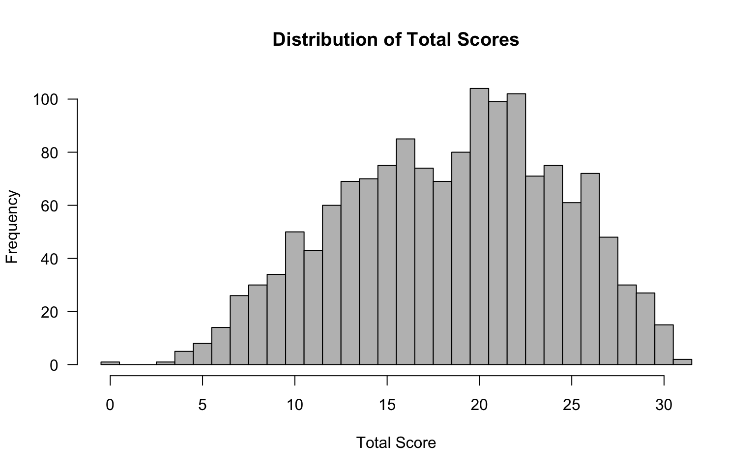

# Check for perfect and zero scores
cat("Number of perfect scores (31):", sum(tot == 31), "\n")

#> Number of perfect scores (31): 2

cat("Number of zero scores (0):", sum(tot == 0), "\n")

#> Number of zero scores (0): 1

Why check for extreme scores? Examinees with perfect or zero scores provide no information for estimating item parameters and can cause estimation problems, particularly for the 3PL model. Watch for these.

15.2 Item Statistics

item_out <- itemAnalysis(d)

Key things to look for in the classical item statistics:

• Item difficulty (\(p\)-value): The proportion of examinees answering correctly. Items with very high or very low \(p\)-values provide little psychometric information and may cause IRT estimation issues.
• Item-total correlations (\(r_{it}\)): A measure of item discrimination in CTT. Low or negative correlations suggest the item is not measuring the same construct as the rest of the test.
• Coefficient alpha: Provides a lower bound on reliability under the assumption of essential tau-equivalence.

A useful way to get an overview of item quality is to plot difficulty against discrimination and apply common screening thresholds. Here we flag items with \(p < .20\) or \(p > .80\) (too hard or too easy) and items with \(r_{it} < .20\) (low discrimination).

# Extract difficulty (item mean) and item-total correlation (point-biserial)
p_vals <- item_out$itemReport$itemMean
r_it   <- item_out$itemReport$pBis
item_nums <- 1:ncol(d)

# Identify flagged items
flag_diff <- p_vals < .20 | p_vals > .80
flag_disc <- r_it < .20
flag_any  <- flag_diff | flag_disc

# Set up plot
plot(p_vals, r_it,
     xlab = "Item Difficulty (p)",
     ylab = expression(Item-Total~Correlation~(r[it])),
     main = "Classical Item Screening",
     xlim = c(0, 1), ylim = c(0, max(r_it) + 0.05),
     pch = 16, col = ifelse(flag_any, "red", "steelblue"),
     cex = 1.2, las = 1)

# Reference lines
abline(v = .20, col = "darkgrey", lty = 2, lwd = 1.5)
abline(v = .80, col = "darkgrey", lty = 2, lwd = 1.5)
abline(h = .20, col = "darkgrey", lty = 2, lwd = 1.5)

# Label flagged items
if (any(flag_any)) {
  text(p_vals[flag_any], r_it[flag_any],
       labels = item_nums[flag_any],
       pos = 3, cex = 0.75, col = "red", font = 2)
}

# Shade the "acceptable" region lightly
rect(.20, .20, .80, par("usr")[4], col = rgb(0, 0.4, 0.8, 0.05), border = NA)

legend("bottomright",
       legend = c("Acceptable", "Flagged"),
       pch = 16, col = c("steelblue", "red"),
       bty = "n", cex = 0.9)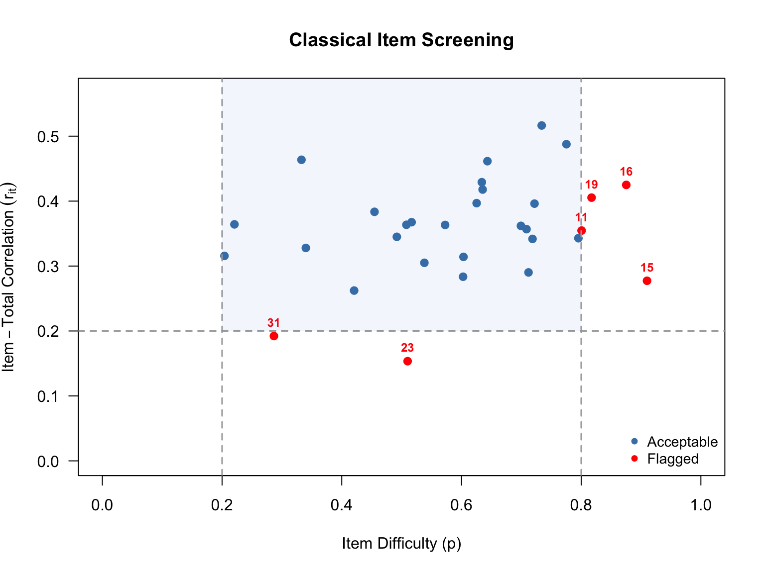

# Build a summary of flagged items
flag_df <- data.frame(
  Item = item_nums[flag_any],
  p = round(p_vals[flag_any], 3),
  r_it = round(r_it[flag_any], 3),
  Reason = ifelse(
    flag_diff[flag_any] & flag_disc[flag_any], "Difficulty & Discrimination",
    ifelse(flag_diff[flag_any], "Difficulty", "Discrimination")
  )
)

if (nrow(flag_df) > 0) {
  kable(flag_df, col.names = c("Item", "$p$", "$r_{it}$", "Reason Flagged"),
        caption = "Items Flagged by Classical Screening Criteria",
        align = "cccc", row.names = FALSE)
} else {
  cat("No items were flagged by the classical screening criteria.\n")
}

Items Flagged by Classical Screening Criteria

Item	\(p\)	\(r_{it}\)	Reason Flagged
11	0.801	0.355	Difficulty
15	0.910	0.277	Difficulty
16	0.875	0.425	Difficulty
19	0.817	0.405	Difficulty
23	0.510	0.154	Discrimination
31	0.287	0.192	Discrimination

The scatterplot above shows each item positioned by its difficulty (\(x\)-axis) and its item-total correlation (\(y\)-axis). The dashed lines mark our screening thresholds: items falling outside the vertical lines (\(p < .20\) or \(p > .80\)) are too hard or too easy for most of the examinee sample, and items falling below the horizontal line (\(r_{it} < .20\)) are not discriminating well between high- and low-performing examinees. Items flagged on one or both criteria are shown in red.

These classical flags give us items to watch closely as we move into IRT modeling. An item that is very difficult with low discrimination in CTT will likely show up again as problematic in the IRT analysis—for example, with an extreme \(b\) parameter, a low \(a\) parameter, or poor item fit. Items flagged here are also prime candidates for convergence trouble in the 3PL model.

15.3 Empirical ICCs

Empirical ICCs plot the proportion correct at each total score level. They give us a visual, model-free look at how each item functions. As you examine these, ask yourself:

• Do the curves seem to have similar slopes? If not, the Rasch model may not be appropriate.
• Is there visual evidence of a lower asymptote (guessing)? If items are multiple-choice and the curves level off above 0 at the low end of the score scale, a 3PL model may be warranted.

scores <- rowSums(d)

op <- par(mfrow = c(11, 3),
          pty = "s",
          mar = c(2.5, 2.5, 2, 0.8),
          cex.main = 0.85,
          cex.axis = 0.7,
          cex.lab = 0.7)

for (k in seq_len(ncol(d))) {
  cttICC(scores = scores, itemVector = d[[k]], plotTitle = paste0("Item ", k))
}

par(op)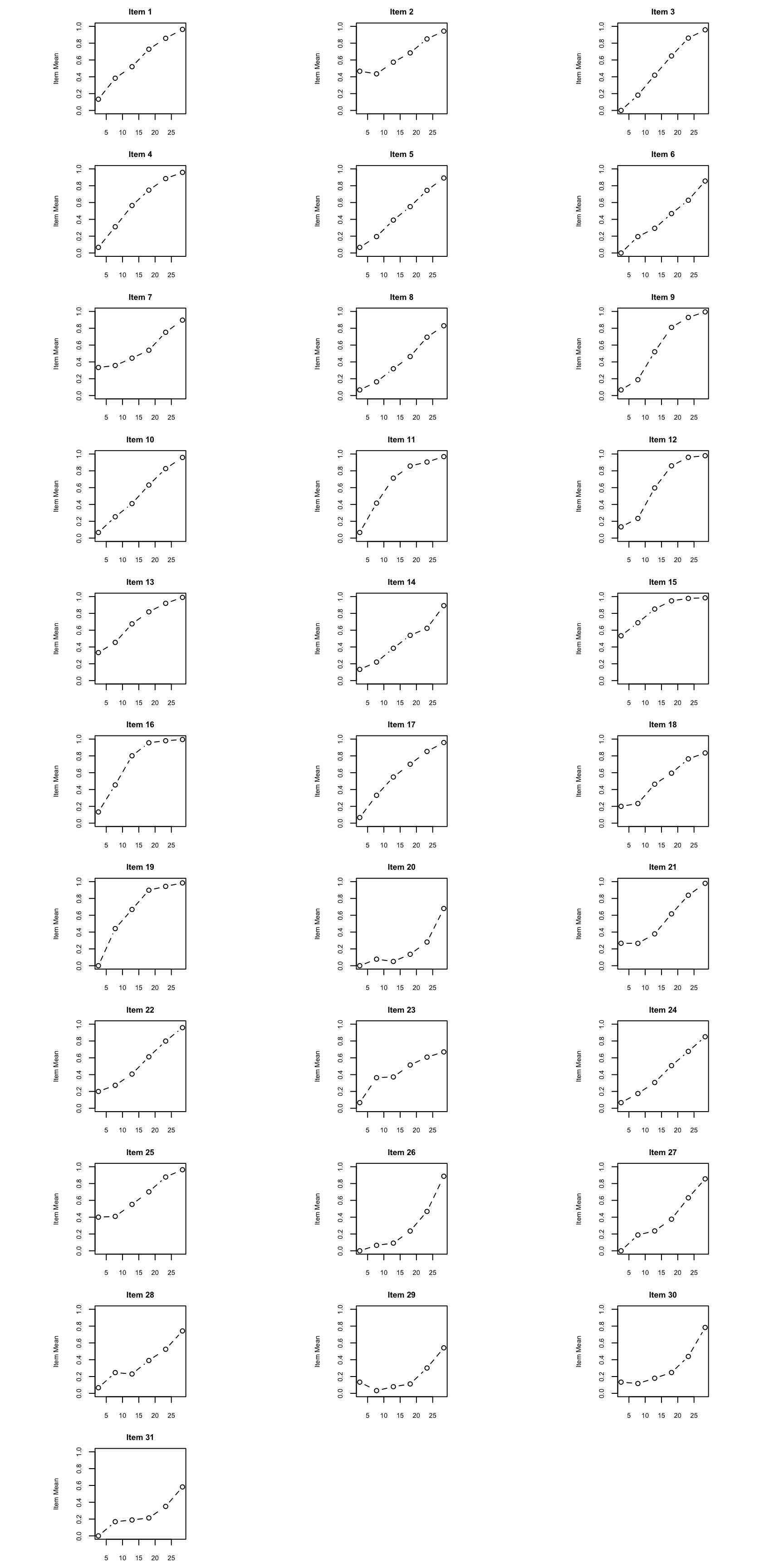

What to look for: Pay particular attention to items where the empirical ICC departs notably from a smooth S-shaped curve. Also look for items where the curve is nearly flat (low discrimination) or where responses from low-ability examinees are well above zero (guessing).

15.4 Parallel Analysis for Unidimensionality

Before fitting unidimensional IRT models, we should check whether a single factor is sufficient. Parallel analysis compares the eigenvalues from the actual data to those from randomly generated data of the same dimensions. If only the first eigenvalue clearly exceeds the random benchmark, the unidimensionality assumption is supported.

pa<-fa.parallel(d, fm="pa", fa="both", main = "Parallel Analysis Scree Plots",
                n.iter=50, SMC=TRUE, ylabel="Eigenvalues of Factors", show.legend=TRUE)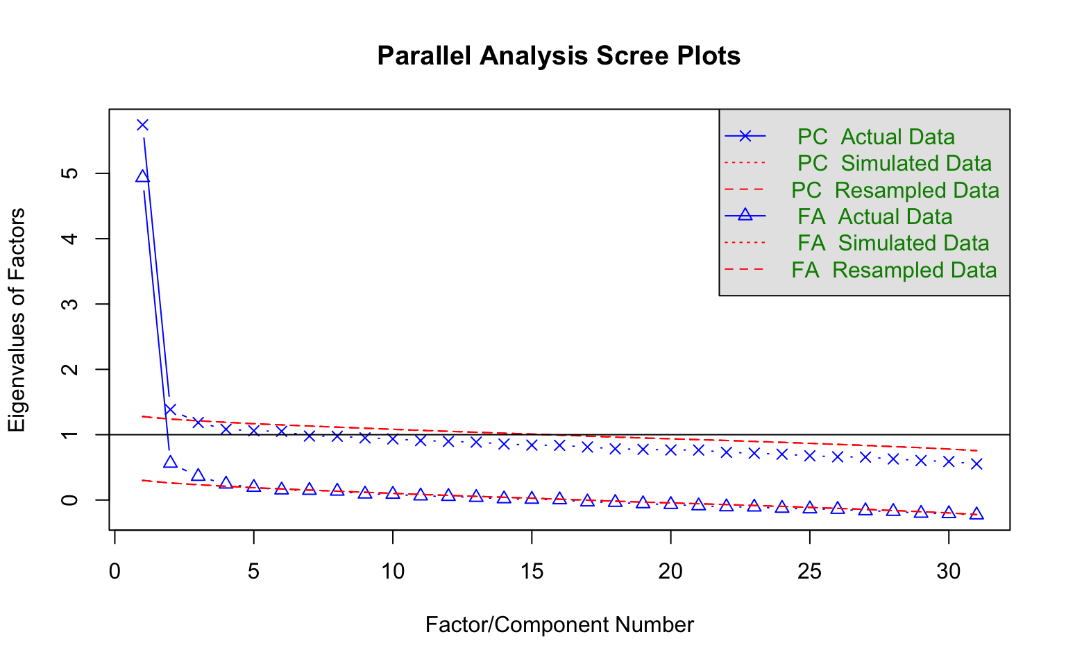

#> Parallel analysis suggests that the number of factors =  4  and the number of components =  2

Interpreting the plot: Focus on the solid blue line (actual eigenvalues) relative to the dashed red line (random data eigenvalues). A clear “elbow” after the first factor, with subsequent factors falling near or below the random line, supports unidimensionality.

15.5 Essentially Unidimensional?

A parallel analysis can be a good way to decide how many factors/dimensions can be considered statistically significant, but it doesn’t necessarily mean that additional dimensions are practically significant. Divgi (1980) takes the difference of the first and second eigenvalues over the difference of the second and third eigenvalues. A cut value of 3 is chosen for the index so that values greater than 3 are considered unidimensional. More generally, Lord (1980) argued that if the first eigenvalue is much larger than the second, it can often be reasonable to treat the test as “essentially unidimensional.” (More sophisticated approaches have been proposed and implemented by Bill Stout with his “DIMTEST” procedure. For details see Nandakumar (1993).)

16 Fitting Competing IRT Models

We fit three unidimensional IRT models, each with progressively more parameters:

Model	Parameters per item	Estimated
1PL (Rasch)	Difficulty (\(b\))	\(b\) only; \(a\) constrained equal across items
2PL	Difficulty (\(b\)), Discrimination (\(a\))	\(a\) and \(b\) freely estimated
3PL	Difficulty (\(b\)), Discrimination (\(a\)), Guessing (\(c\))	\(a\), \(b\), and \(c\) freely estimated

We request SE = TRUE so that standard errors are computed for all parameter estimates.

mod1 <- mirt(d, 1, itemtype = "Rasch", SE = TRUE)
mod2 <- mirt(d, 1, itemtype = "2PL", SE = TRUE)

The 1PL and 2PL converge without issue. Now the 3PL:

mod3 <- mirt(d, 1, itemtype = "3PL", SE = TRUE)

#> Warning: EM cycles terminated after 500 iterations.

Notice the warning: the EM algorithm reached its default limit of 500 iterations without converging. This is common with the 3PL because the guessing parameter (\(c\)) is often poorly identified, making the likelihood surface flat in certain regions of the parameter space.

16.1 Dealing with Convergence Issues

The 3PL model, in particular, can be difficult to estimate because the guessing parameter (\(c\)) is often poorly identified. If the model does not converge—as is the case with this data example—here are two strategies you can apply.

Strategy 1: Increase the number of EM cycles.

mod3 <- mirt(d, 1, itemtype = "3PL", SE = TRUE, technical = list(NCYCLES = 2000))

Strategy 2: Remove problematic items. If you identified items from the classical diagnostics that have very low \(p\)-values, extremely low discrimination, or other anomalies, try removing them.

# Example: if item 23 was flagged as problematic
d2 <- d[, -23]
mod3r <- mirt(d2, 1, itemtype = "3PL", SE = TRUE)

Note that Strategy 2 changes the item set, so the reduced model is not directly comparable to the full models via likelihood ratio tests. We will focus on the full 31-item models going forward (based on using mod3 with increased EM cycles which leads to convergence).

16.2 Parameter Estimates

Let’s examine the 3PL parameter estimates and their standard errors. Here is what the default coef() output looks like for the first five items:

coef(mod3, IRTpars = TRUE, printSE = TRUE)[1:5]

#> $V1
#>             a          b         g  u
#> par 1.3010094 -0.4065298 0.2714853  1
#> SE  0.2256101  0.2861556 0.1056328 NA
#> 
#> $V2
#>             a         b          g  u
#> par 1.5478092 0.1760955 0.47146339  1
#> SE  0.3015103 0.1954730 0.05509958 NA
#> 
#> $V3
#>             a          b          g  u
#> par 1.4500298 -0.4982353 0.03821073  1
#> SE  0.1808243  0.1750681 0.08683516 NA
#> 
#> $V4
#>              a          b           g  u
#> par 1.17041672 -1.0178820 0.005665404  1
#> SE  0.09983055  0.1300436 0.052548495 NA
#> 
#> $V5
#>              a           b           g  u
#> par 0.93275396 -0.36490298 0.001074912  1
#> SE  0.07590473  0.07379082 0.009544876 NA

This is informative but unwieldy for 31 items. Let’s create a more compact summary table.

# Extract IRT-parameterized coefficients with SEs
pars_list <- coef(mod3, IRTpars = TRUE, printSE = TRUE)

# Build a data frame from the item-level coefficient matrices
# Each element is a matrix with rows: par, SE (and possibly CI bounds)
item_names <- names(pars_list)
# Remove the GroupPars element
item_names <- item_names[item_names != "GroupPars"]

param_df <- do.call(rbind, lapply(item_names, function(nm) {
  mat <- pars_list[[nm]]
  data.frame(
    Item = nm,
    a = mat["par", "a"],
    SE_a = mat["SE", "a"],
    b = mat["par", "b"],
    SE_b = mat["SE", "b"],
    c = mat["par", "g"],
    SE_c = mat["SE", "g"],
    row.names = NULL
  )
}))

kable(param_df, digits = 3, align = "lcccccc",
      col.names = c("Item", "$a$", "$SE(a)$", "$b$", "$SE(b)$", "$c$", "$SE(c)$"),
      caption = "3PL Item Parameter Estimates and Standard Errors")

3PL Item Parameter Estimates and Standard Errors

Item	\(a\)	\(SE(a)\)	\(b\)	\(SE(b)\)	\(c\)	\(SE(c)\)
V1	1.301	0.226	-0.407	0.286	0.271	0.106
V2	1.548	0.302	0.176	0.195	0.471	0.055
V3	1.450	0.181	-0.498	0.175	0.038	0.087
V4	1.170	0.100	-1.018	0.130	0.006	0.053
V5	0.933	0.076	-0.365	0.074	0.001	0.010
V6	0.892	0.177	0.088	0.341	0.015	0.125
V7	1.888	0.353	0.643	0.113	0.417	0.034
V8	1.103	0.176	0.267	0.187	0.117	0.070
V9	1.988	0.210	-0.767	0.118	0.048	0.069
V10	1.634	0.234	-0.087	0.148	0.229	0.062
V11	1.123	0.097	-1.520	0.133	0.005	0.041
V12	1.879	0.140	-1.022	0.068	0.002	0.022
V13	1.200	0.209	-1.140	0.470	0.193	0.205
V14	0.817	0.168	-0.039	0.423	0.062	0.139
V15	1.297	0.249	-2.016	0.781	0.213	0.429
V16	1.932	0.202	-1.550	0.171	0.013	0.124
V17	1.017	0.084	-0.995	0.101	0.003	0.023
V18	0.780	0.075	-0.596	0.143	0.004	0.040
V19	1.471	0.116	-1.389	0.090	0.002	0.018
V20	1.991	0.262	1.262	0.075	0.060	0.015
V21	2.381	0.319	0.091	0.087	0.303	0.037
V22	1.528	0.239	-0.071	0.173	0.217	0.071
V23	0.338	0.068	-0.056	0.617	0.011	0.097
V24	1.005	0.168	0.053	0.247	0.052	0.094
V25	1.897	0.356	0.045	0.163	0.448	0.054
V26	2.292	0.308	0.752	0.059	0.078	0.022
V27	1.539	0.224	0.592	0.100	0.165	0.039
V28	1.023	0.208	1.066	0.165	0.185	0.052
V29	1.494	0.214	1.520	0.105	0.053	0.017
V30	1.802	0.299	1.083	0.083	0.157	0.026
V31	1.397	0.338	1.825	0.169	0.184	0.026

What to look for in the parameter table:

• Discrimination (\(a\)): Values near or below 0.5 suggest an item is weakly related to the measured trait. Very high values (\(> 3\)) may indicate estimation instability.
• Difficulty (\(b\)): Values far outside the range of \(\theta\) (e.g., \(|b| > 3\)) suggest the item is too easy or too hard for the population.
• Guessing (\(c\)): For a 4-option multiple-choice item, values near 0.25 are consistent with chance; values near 0 suggest no guessing. Large standard errors on \(c\) indicate the parameter is poorly estimated.

Applying these guidelines to our 31 items:

Discrimination. Most items have discrimination values in the range of about 0.8 to 2.4, with a median around 1.4—indicating generally good discriminating power. The clear outlier is Item 23 (\(a = 0.34\)), which is well below the 0.5 threshold. This is the same item we flagged in the classical analysis for low item-total correlation, and it confirms that Item 23 is contributing very little information to the measurement of the latent trait.

Difficulty. The \(b\) parameters span a range from roughly \(-2.0\) to \(+1.8\), which is well within \(\pm 3\) and suggests the items provide good coverage across the ability scale. The easier items (e.g., Items 11, 15, 16, and 19 with \(b < -1.3\)) target lower-ability examinees, while the harder items (e.g., Items 20, 29, and 31 with \(b > 1.2\)) target higher-ability examinees. None of the \(b\) estimates are extreme enough to raise concern about estimation instability.

Guessing. This is where the most interesting patterns emerge. About a third of the items have \(c\) estimates near zero (e.g., Items 4, 5, 11, 12, 17, 18, 19), suggesting no appreciable guessing—these items might be well-served by a 2PL model. On the other hand, three items stand out with notably high \(c\) values: Item 2 (\(c = .47\)), Item 7 (\(c = .42\)), and Item 25 (\(c = .45\)). These are above what we would expect from random guessing on a 4-option item (.25), which is unusual and may indicate either that the incorrect options are not functioning as intended, or that there is some other source of correct responses among low-ability examinees.

Standard errors. The SEs on \(c\) deserve particular attention. For several items the SE on \(c\) is quite large relative to the estimate itself—for example, Item 15 (\(c = .21\), \(SE = .43\)) and Item 13 (\(c = .19\), \(SE = .21\)). These SEs indicate that the guessing parameter is essentially unidentified for those items. This is a common issue with the 3PL model and one reason many practitioners prefer the 2PL unless guessing is clearly and consistently present.

17 Overall Model Comparison

When comparing nested models, we can use the likelihood ratio test (LRT) implemented through anova() in mirt. This tests whether the additional parameters in the more complex model lead to a statistically significant improvement in fit.

# Compare 1PL to 2PL
anova(mod1, mod2)

#>           AIC    SABIC       HQ      BIC    logLik      X2 df p
#> mod1 51392.88 51461.25 51456.22 51562.90 -25664.44             
#> mod2 50914.97 51047.44 51037.69 51244.39 -25395.49 537.907 30 0

The 1PL is nested within the 2PL (the 1PL constrains all \(a\) parameters to be equal). A significant result suggests the 2PL (which allows discrimination to vary) fits the data better. Indeed, that that’s the case in this example (note that p <.01 in the far right column of mod2).

# Compare 2PL to 3PL
anova(mod2, mod3)

#>           AIC    SABIC       HQ      BIC    logLik      X2 df p
#> mod2 50914.97 51047.44 51037.69 51244.39 -25395.49             
#> mod3 50826.81 51025.51 51010.89 51320.94 -25320.41 150.162 31 0

The 2PL is nested within the 3PL (the 2PL constrains all \(c = 0\)). A significant result (as found in this example) suggests guessing is present and the 3PL provides a better fit relative to the 2PL (this time note that p <.01 in the far right column of mod3)

Caution: The LRT tells us about relative fit between two models. It does not tell us whether either model fits the data well in an absolute sense. We need item-level fit statistics for that.

Also examine the AIC and BIC values reported in the output. These information criteria penalize model complexity differently:

• AIC penalizes more lightly and tends to favor more complex models.
• BIC penalizes more heavily (as a function of sample size) and tends to favor simpler models.
• When AIC and BIC disagree, the “truth” often lies in the middle, and other evidence (item fit, empirical plots) should guide the decision.

18 Item Fit Statistics

Item fit statistics assess whether each individual item conforms to the fitted model. This is where we move from “which model is best overall?” to “which specific items don’t fit?”

18.1 Yen’s Q1 Statistic

Yen’s (1981) Q1 statistic is one of the oldest and most widely used item fit statistics. It works by:

1. Sorting examinees into \(G\) groups (bins) based on their estimated \(\theta\).
2. Computing the observed and expected proportion correct within each bin.
3. Comparing observed and expected proportions via a Pearson-type \(\chi^2\) statistic.

Under the null hypothesis (item fits the model), Q1 approximately follows a \(\chi^2\) distribution with \(G - m\) degrees of freedom, where \(m\) is the number of item parameters.

Known limitation: Q1 has inflated Type I error rates, especially for shorter tests (Orlando & Thissen, 2000). This means it may flag items as misfitting even when they actually fit the model. We will return to this issue below.

f1 <- itemfit(mod1, fit_stats = c("X2"), group.bins = 10, method = "EAP")
f2 <- itemfit(mod2, fit_stats = c("X2"), group.bins = 10, method = "EAP")
f3 <- itemfit(mod3, fit_stats = c("X2"), group.bins = 10, method = "EAP")

# Compare p-values across models
# Helper: format p-value, bolding those < .05
bold_sig <- function(p) {
  ifelse(p < .05,
         paste0("**", formatC(p, digits = 3, format = "f"), "**"),
         formatC(p, digits = 3, format = "f"))
}

Yen <- data.frame(
  Item = f1$item,
  p_1PL = bold_sig(f1$p.X2),
  p_2PL = bold_sig(f2$p.X2),
  p_3PL = bold_sig(f3$p.X2)
)

kable(Yen, col.names = c("Item", "$p$ (1PL)", "$p$ (2PL)", "$p$ (3PL)"),
      caption = "Yen's Q1 p-values Across Models (significant values in bold)",
      align = "lccc")

Yen’s Q1 p-values Across Models (significant values in bold)

Item	\(p\) (1PL)	\(p\) (2PL)	\(p\) (3PL)
V1	0.287	0.248	0.334
V2	0.391	0.089	0.187
V3	0.000	0.037	0.104
V4	0.002	0.047	0.095
V5	0.655	0.010	0.001
V6	0.530	0.309	0.432
V7	0.007	0.000	0.062
V8	0.230	0.022	0.013
V9	0.000	0.008	0.009
V10	0.001	0.035	0.198
V11	0.000	0.087	0.067
V12	0.000	0.010	0.002
V13	0.065	0.541	0.308
V14	0.070	0.016	0.022
V15	0.023	0.042	0.153
V16	0.000	0.023	0.062
V17	0.422	0.027	0.049
V18	0.268	0.014	0.066
V19	0.000	0.328	0.164
V20	0.000	0.000	0.010
V21	0.000	0.001	0.157
V22	0.060	0.025	0.500
V23	0.000	0.557	0.309
V24	0.044	0.173	0.070
V25	0.087	0.008	0.177
V26	0.000	0.000	0.003
V27	0.004	0.011	0.240
V28	0.000	0.000	0.002
V29	0.053	0.023	0.203
V30	0.001	0.004	0.272
V31	0.000	0.019	0.227

Interpreting the table: Items with small \(p\)-values (e.g., \(< .05\)) show evidence of misfit under that model. Compare across columns: an item that misfits under the 1PL but fits under the 2PL likely has unusual discrimination. An item that misfits under the 2PL but fits under the 3PL may have a guessing component.

18.2 Chalmers’ PV-Q1 Statistic

Chalmers and Ng (2017) proposed the PV-Q1 as an improvement to Q1. The key insight is that Q1 treats estimated \(\hat{\theta}\) values as known when forming groups, ignoring the uncertainty in \(\theta\) estimation. This is a major source of the inflated Type I error rates.

How PV-Q1 works:

1. Draw plausible values (PVs) of \(\theta\) from each examinee’s posterior distribution.
2. Form groups based on these PVs (instead of point estimates).
3. Compute the Q1 statistic using the PV-based grouping.
4. Repeat this process many times and average the resulting statistics.

The PV-Q1 statistic has Type I error rates much closer to the nominal level, especially for shorter tests where \(\theta\) estimation is less precise.

f3n <- itemfit(mod3, fit_stats = c("X2", "PV_Q1"), group.bins = 10, method = "EAP")

compare <- data.frame(
  Item = f3n$item,
  p_Q1 = bold_sig(f3n$p.X2),
  p_PV_Q1 = bold_sig(f3n$p.PV_Q1)
)

kable(compare, col.names = c("Item", "$p$ (Q1)", "$p$ (PV-Q1)"),
      caption = "Q1 vs. PV-Q1 p-values for the 3PL Model (significant values in bold)",
      align = "lcc")

Q1 vs. PV-Q1 p-values for the 3PL Model (significant values in bold)

Item	\(p\) (Q1)	\(p\) (PV-Q1)
V1	0.334	0.345
V2	0.187	0.305
V3	0.104	0.548
V4	0.095	0.433
V5	0.001	0.386
V6	0.432	0.399
V7	0.062	0.312
V8	0.013	0.154
V9	0.009	0.218
V10	0.198	0.426
V11	0.067	0.397
V12	0.002	0.039
V13	0.308	0.295
V14	0.022	0.370
V15	0.153	0.110
V16	0.062	0.264
V17	0.049	0.371
V18	0.066	0.341
V19	0.164	0.233
V20	0.010	0.290
V21	0.157	0.283
V22	0.500	0.433
V23	0.309	0.143
V24	0.070	0.201
V25	0.177	0.379
V26	0.003	0.250
V27	0.240	0.369
V28	0.002	0.079
V29	0.203	0.257
V30	0.272	0.325
V31	0.227	0.511

What to expect: You will often see that PV-Q1 produces larger \(p\)-values (fewer rejections) than Q1. Items flagged by Q1 but not by PV-Q1 were likely false positives. Items flagged by both statistics provide stronger evidence of genuine misfit.

18.3 Empirical Fit Plots

Numerical fit statistics are useful, but always supplement them with visual inspection. Empirical fit plots overlay the model-predicted ICC on the empirical (observed) proportions at each ability level. These plots make it easy to see where and how the model fails to fit.

# Empirical fit plot using Q1 grouping
itemfit(mod3, fit_stats = c("X2"), group.bins = 10, empirical.plot = 14, xlim = c(-3, 3))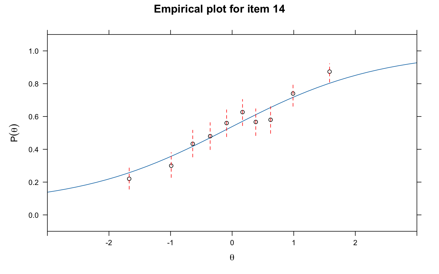

# Empirical fit plot using PV-Q1 grouping
itemfit(mod3, fit_stats = c("PV_Q1"), group.bins = 10, empirical.plot = 14, xlim = c(-3, 3))

What to look for:

• Systematic departures: The observed points consistently fall above or below the predicted curve in a region. This suggests the model is wrong in that region of \(\theta\).
• Differences between Q1 and PV-Q1 groupings: The PV-Q1 version may show less apparent misfit because the grouping better accounts for \(\theta\) uncertainty.

You can change the item number in empirical.plot to examine any item. It is good practice to inspect items flagged as misfitting, as well as a sample of well-fitting items, to calibrate your visual judgement.

To view all 31 empirical fit plots at once, we can save them as a multi-page PDF (one item per page). Note that itemfit() with empirical.plot creates a standalone plot on each call, so par(mfrow) does not work with it — a PDF with one plot per page is the way to go.

pdf("empirical_fit_plots_3PL.pdf", width = 7, height = 5)

for (k in seq_len(ncol(d))) {
  # itemfit returns a lattice (trellis) object, which must be explicitly
  # printed to render inside a loop or non-interactive device
  print(itemfit(mod3, fit_stats = c("X2"), group.bins = 10,
                empirical.plot = k, xlim = c(-3, 3)))
}

invisible(dev.off())

19 Person Fit

Person fit statistics identify examinees whose response patterns are inconsistent with the model. The most common statistic is the standardized log-likelihood ratio, \(l_z\) (Drasgow et al., 1985).

How \(l_z\) works: For each examinee, it computes the log-likelihood of their observed response pattern given the model and their estimated \(\theta\), and then standardizes this value. Large negative values of \(l_z\) indicate aberrant response patterns—the examinee’s responses are less likely than the model predicts for someone at their ability level.

Common sources of person misfit include:

• Guessing/random responding: Low-ability examinees who get difficult items correct by chance.
• Carelessness: High-ability examinees who miss easy items.
• Cheating/copying: Response patterns that reflect another examinee’s ability level.
• Speededness: Examinees who run out of time and miss items at the end regardless of difficulty.

Let’s look at the \(l_z\) statistics for the first 20 examinees.

lz <- personfit(mod3)
head(lz, 20)

#>       outfit   z.outfit     infit     z.infit          Zh
#> 1  0.7462836 -0.9432010 0.8016347 -1.23808052  1.13835976
#> 2  0.8841978 -0.4300856 0.9281965 -0.44253447  0.47109818
#> 3  0.8238428 -0.6936679 0.9285431 -0.42107117  0.57626619
#> 4  0.8492439 -0.1374976 1.0197154  0.16199785  0.04635475
#> 5  1.3979418  1.6397305 1.2975157  1.94840614 -2.01255039
#> 6  3.3923110  2.0785375 0.9978132  0.08884632 -0.60167773
#> 7  0.7655236 -0.9716392 0.8544809 -0.95269532  0.97477333
#> 8  1.1460655  0.4710558 1.1589329  0.79604835 -0.70435368
#> 9  1.2677980  0.8963200 1.3500942  1.81589992 -1.67845829
#> 10 0.5540594 -1.1891524 0.6902171 -1.63912196  1.47765786
#> 11 0.6162276 -1.0158118 0.7368906 -1.37733714  1.27958831
#> 12 1.5595572  0.9898273 0.9960123  0.06486048 -0.31359342
#> 13 1.1731188  0.8238607 1.1020870  0.77120723 -0.79299085
#> 14 1.2924299  0.7994144 1.2698409  1.28809470 -1.27744204
#> 15 0.5380617 -0.6597944 0.8080736 -0.73987396  0.86622976
#> 16 0.9716941  0.2935635 0.9067865 -0.18941823  0.07501934
#> 17 1.2350659  0.8795428 1.2434877  1.40115958 -1.32314873
#> 18 1.0097173  0.2274315 0.9643942 -0.06167773  0.06706602
#> 19 0.2896286 -0.5134008 0.6690958 -0.81174926  0.91935734
#> 20 0.8704179 -0.4089528 0.9696080 -0.13034675  0.29007570

hist(lz$Zh, breaks = 40, main = "Distribution of Zh (Standardized Person Fit)",
     xlab = expression(Z[h]), col = "grey", las = 1)
abline(v = -2, col = "red", lty = 2, lwd = 2)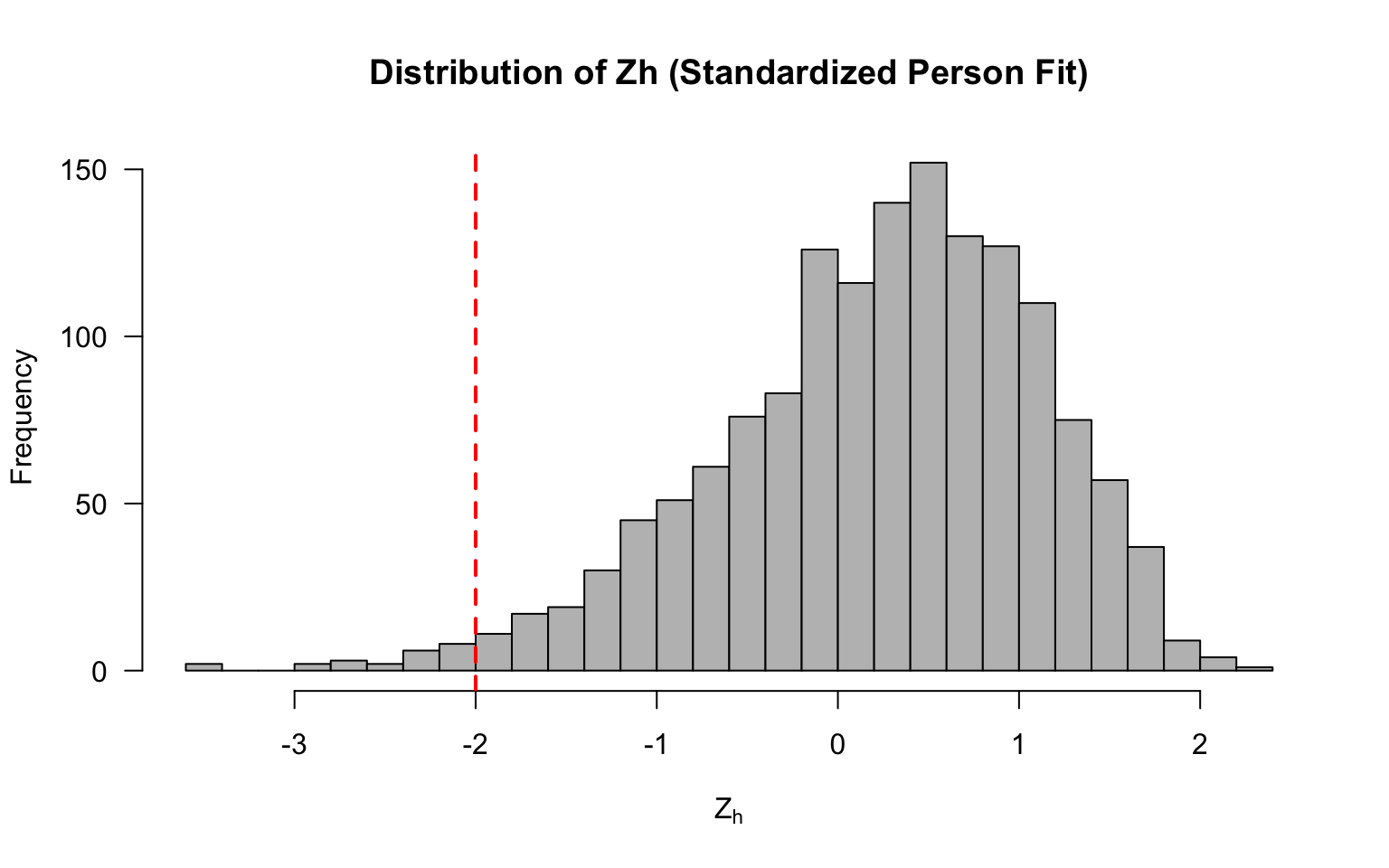

Now let’s flag any examinees with values < -2.

# Flag examinees with Zh < -2 (common cutoff)
flagged <- sum(lz$Zh < -2, na.rm = TRUE)
cat("Number of examinees flagged (Zh < -2):", flagged, "\n")

#> Number of examinees flagged (Zh < -2): 23

cat("Percentage flagged:", round(100 * flagged / nrow(d), 1), "%\n")

#> Percentage flagged: 1.5 %

Interpreting person fit: The \(Z_h\) statistic is approximately standard normal under the null hypothesis. Values below \(-2\) are commonly used as a flag. However, be cautious about over-interpreting person fit for individual examinees—it is more useful for identifying systematic patterns (e.g., a large proportion of misfitting examinees may indicate a model problem rather than examinee problems).

20 Checking Local Independence and Parameter Invariance

20.1 Local Independence: Yen’s Q3

Local independence means that after conditioning on \(\theta\), the residual correlations between item pairs should be approximately zero. Yen’s (1993) Q3 statistic assesses this by computing correlations between item residuals.

Procedure:

1. Compute standardized residuals: \(e_{ij} = x_{ij} - P_j(\hat{\theta}_i)\), where \(x_{ij}\) is the observed response and \(P_j(\hat{\theta}_i)\) is the model-predicted probability.
2. Compute the correlation matrix of these residuals across all item pairs.
3. Flag item pairs with residual correlations that are “too large.”

Note: Because residuals must sum to a constant given a fixed \(\theta\), the expected average Q3 correlation is slightly negative (approximately \(-1/(J-1)\) for \(J\) items). So a value of \(0.00\) is already slightly above average. Various thresholds have been proposed for flagging LD; a common rule of thumb is to flag pairs where \(|Q3| > .20\) above the average Q3 value.

# Compute the Q3 matrix (suppress the printed matrix)
Q3_mat <- residuals(mod3, type = "Q3", method = "EAP")

# Summary statistics for the lower triangle
lower_tri <- Q3_mat[lower.tri(Q3_mat)]
cat("Mean Q3 (lower triangle):", round(mean(lower_tri), 4), "\n")

#> Mean Q3 (lower triangle): -0.0264

cat("SD of Q3 values:", round(sd(lower_tri), 4), "\n")

#> SD of Q3 values: 0.0349

cat("Range:", round(min(lower_tri), 4), "to", round(max(lower_tri), 4), "\n")

#> Range: -0.1187 to 0.0832

Rather than printing the full 31 \(\times\) 31 matrix, a heatmap of the lower triangle makes it easy to spot clusters of local dependence at a glance.

# Mask upper triangle and diagonal for plotting
Q3_plot <- Q3_mat
Q3_plot[upper.tri(Q3_plot, diag = TRUE)] <- NA

# Set up color palette: blue (negative) -> white (zero) -> red (positive)
n_colors <- 100
breaks <- seq(-0.3, 0.4, length.out = n_colors + 1)
colors <- colorRampPalette(c("steelblue", "white", "firebrick"))(n_colors)

par(mar = c(5, 5, 3, 6))
image(1:31, 1:31, t(Q3_plot[31:1, ]),
      col = colors, breaks = breaks,
      xlab = "Item", ylab = "Item",
      main = "Q3 Residual Correlations (Lower Triangle)",
      axes = FALSE, las = 1)
axis(1, at = seq(1, 31, by = 5), cex.axis = 0.8)
axis(2, at = seq(1, 31, by = 5), labels = rev(seq(1, 31, by = 5)), cex.axis = 0.8)

# Add a color legend
legend_y <- seq(5, 27, length.out = n_colors)
for (i in seq_len(n_colors)) {
  rect(33, legend_y[i], 34, legend_y[i + 1],
       col = colors[i], border = NA, xpd = TRUE)
}
text(35, legend_y[1], round(breaks[1], 2), cex = 0.7, xpd = TRUE)
text(35, legend_y[n_colors], round(breaks[n_colors + 1], 2), cex = 0.7, xpd = TRUE)
text(35, legend_y[round(n_colors / 2)], "0.00", cex = 0.7, xpd = TRUE)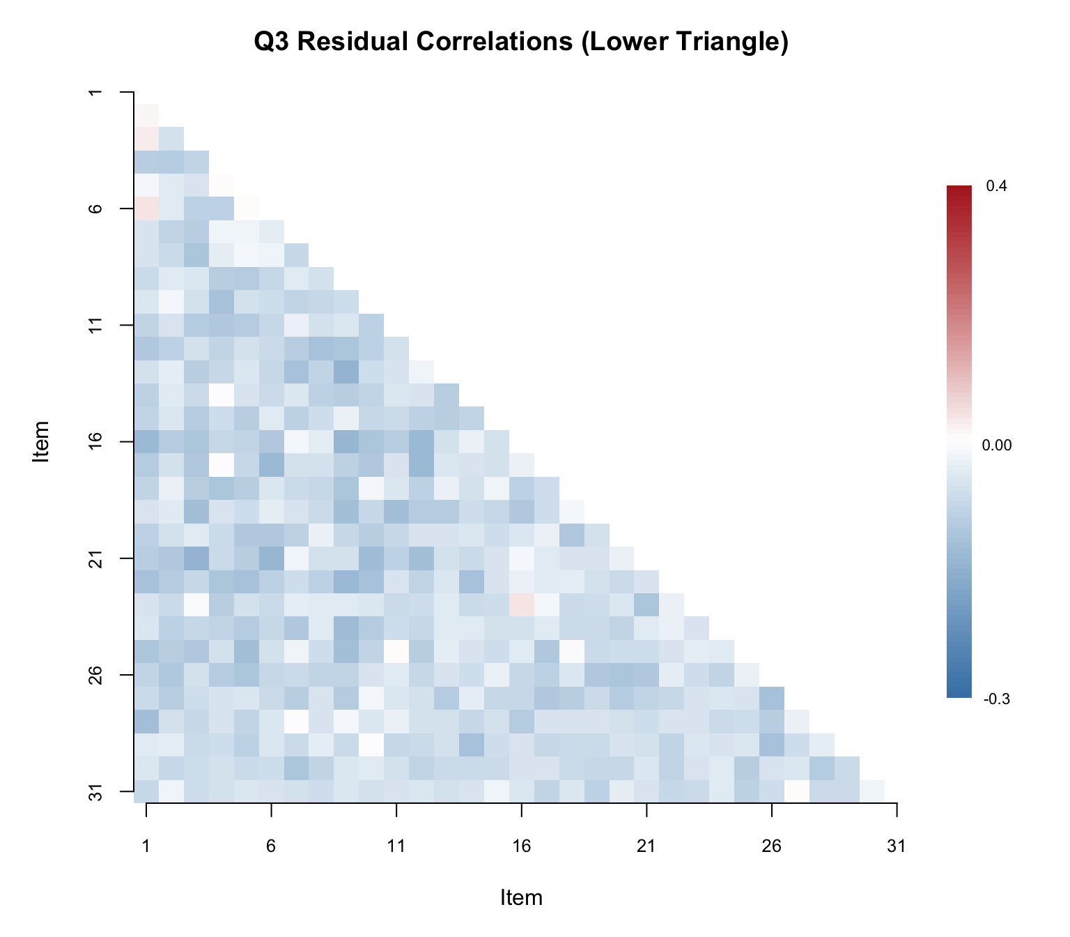

Now let’s identify the specific item pairs that exceed the \(.20\) threshold.

# Build a table of flagged item pairs (Q3 > .20)
flagged_pairs <- which(Q3_mat > .20 & lower.tri(Q3_mat), arr.ind = TRUE)

if (nrow(flagged_pairs) > 0) {
  flag_df <- data.frame(
    Item_1 = colnames(Q3_mat)[flagged_pairs[, 2]],
    Item_2 = rownames(Q3_mat)[flagged_pairs[, 1]],
    Q3 = round(Q3_mat[flagged_pairs], 3)
  )
  flag_df <- flag_df[order(-flag_df$Q3), ]

  cat("Number of item pairs with Q3 > .20:", nrow(flag_df),
      "out of", choose(ncol(d), 2), "total pairs\n\n")

  kable(flag_df, col.names = c("Item 1", "Item 2", "Q3"),
        caption = "Item Pairs Flagged for Local Dependence (Q3 > .20)",
        align = "llc", row.names = FALSE)
} else {
  cat("No item pairs exceeded the Q3 > .20 threshold.\n")
}

#> No item pairs exceeded the Q3 > .20 threshold.

Interpreting Q3: A small number of flagged pairs is not necessarily alarming—some false positives are expected. However, if many pairs are flagged, or if the flagged pairs cluster among a subset of items, this suggests local dependence that could bias parameter estimates. Common causes of LD include:

• Items that share a common stimulus (e.g., a reading passage).
• Items that test the same narrow sub-skill.
• Testlet structures (groups of items about the same scenario).

20.2 Parameter Invariance

A hallmark property of IRT is that item parameters should be invariant across samples from the same population (up to sampling variability and a linear transformation). We can check this empirically by splitting the sample, estimating models separately, and comparing the resulting parameter estimates.

# Split sample in half (assuming random ordering)
samp1 <- d[1:750, ]
samp2 <- d[751:1500, ]

# Fit 3PL to each subsample
est1 <- mirt(samp1, 1, itemtype = "3PL")

est2 <- mirt(samp2, 1, itemtype = "3PL")

# Extract parameters
coef1 <- coef(est1, IRTpars = TRUE, simplify = TRUE)$items
coef2 <- coef(est2, IRTpars = TRUE, simplify = TRUE)$items

r_a <- round(cor(coef1[, "a"], coef2[, "a"]), 3)
r_b <- round(cor(coef1[, "b"], coef2[, "b"]), 3)
r_g <- round(cor(coef1[, "g"], coef2[, "g"]), 3)

cat("Correlation of a estimates:", r_a, "\n")

#> Correlation of a estimates: 0.605

cat("Correlation of b estimates:", r_b, "\n")

#> Correlation of b estimates: 0.911

cat("Correlation of g estimates:", r_g, "\n")

#> Correlation of g estimates: 0.384

par(mfrow = c(3, 1), mar = c(4.5, 4.5, 3, 1))

# Compute shared axis limits for each parameter
lim_a <- range(c(coef1[, "a"], coef2[, "a"]))
lim_b <- range(c(coef1[, "b"], coef2[, "b"]))
lim_g <- range(c(coef1[, "g"], coef2[, "g"]))

# Discrimination (a)
plot(coef1[, "a"], coef2[, "a"],
     xlab = "Sample 1 (a)", ylab = "Sample 2 (a)",
     xlim = lim_a, ylim = lim_a,
     main = "Discrimination Invariance", pch = 16, col = "steelblue", cex = 1.2)
abline(0, 1, col = "red", lty = 2)
text(coef1[, "a"], coef2[, "a"], labels = rownames(coef1), pos = 3, cex = 0.9)
legend("topleft", legend = paste0("r = ", r_a), bty = "n", cex = 1.1)

# Difficulty (b)
plot(coef1[, "b"], coef2[, "b"],
     xlab = "Sample 1 (b)", ylab = "Sample 2 (b)",
     xlim = lim_b, ylim = lim_b,
     main = "Difficulty Invariance", pch = 16, col = "steelblue", cex = 1.2)
abline(0, 1, col = "red", lty = 2)
text(coef1[, "b"], coef2[, "b"], labels = rownames(coef1), pos = 3, cex = 0.9)
legend("topleft", legend = paste0("r = ", r_b), bty = "n", cex = 1.1)

# Guessing (c)
plot(coef1[, "g"], coef2[, "g"],
     xlab = "Sample 1 (c)", ylab = "Sample 2 (c)",
     xlim = lim_g, ylim = lim_g,
     main = "Guessing Invariance", pch = 16, col = "steelblue", cex = 1.2)
abline(0, 1, col = "red", lty = 2)
text(coef1[, "g"], coef2[, "g"], labels = rownames(coef1), pos = 3, cex = 0.9)
legend("topleft", legend = paste0("r = ", r_g), bty = "n", cex = 1.1)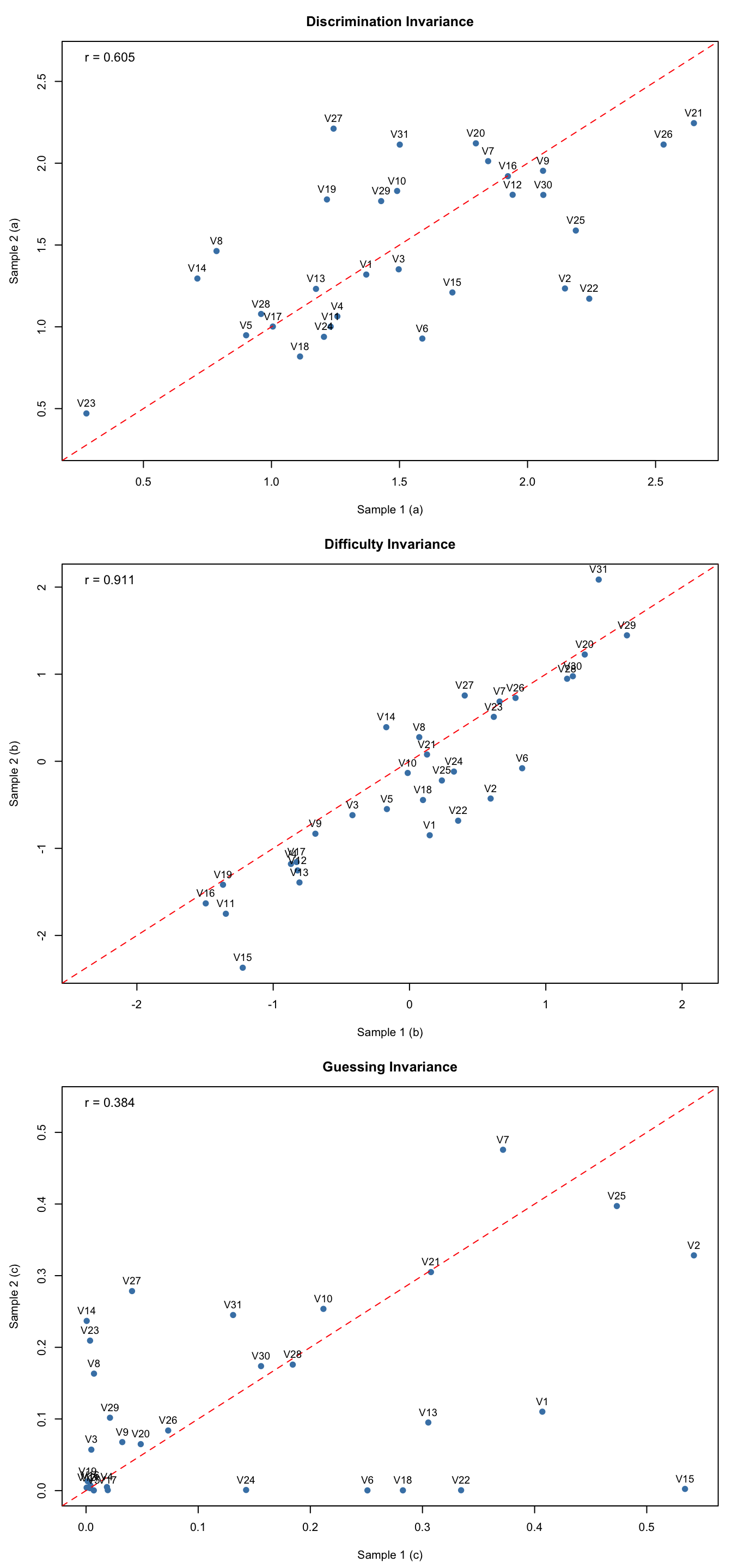

par(mfrow = c(1, 1))

Interpreting invariance plots: Points should cluster near the identity line (red dashed). Look for:

• Overall trend: High correlations (especially for \(b\) parameters) support invariance.
• Outliers: Items that deviate notably from the line may have unstable parameter estimates.
• Parameter-specific patterns: Difficulty (\(b\)) typically shows the best invariance. Discrimination (\(a\)) may show more variability. Guessing (\(c\)) is notoriously hard to estimate and often shows the weakest invariance—this is one reason many practitioners prefer the 2PL over the 3PL unless there is strong evidence of guessing. Another strategy is to place constraints or to fix guessing parameters to values based on the number of item response options.

21 Summary and Recommendations

21.1 Practical Workflow for Evaluating Fit

1. Start with the data. Compute classical item statistics and plot empirical ICCs. Flag items with unusual \(p\)-values, low discrimination, or irregular ICC shapes.

2. Check dimensionality. Run parallel analysis. If unidimensionality is supported (additional factors are not statistically or practically significant), proceed with unidimensional models. If not, consider multidimensional models or bifactor models.

3. Fit competing models. Estimate 1PL, 2PL, and 3PL. Use likelihood ratio tests and information criteria (AIC, BIC) to compare overall fit.

4. Evaluate item fit. Use multiple statistics:

   • PV-Q1 (Chalmers & Ng, 2017) provides better Type I error control than the original Q1.
   • S-\(\chi^2\) (Orlando & Thissen, 2000) is another well-regarded alternative (available in mirt as "S_X2").
   • Always supplement statistics with empirical fit plots. A picture is worth a thousand \(\chi^2\) values.

5. Check person fit. Identify aberrant response patterns. Consider whether misfit is concentrated in a particular group of examinees.

6. Verify assumptions. Use Q3 to check local independence. Check parameter invariance by fit the model to unique groups of test-takers.

21.2 A Note on Statistical vs. Practical Significance

With large samples (\(N > 1{,}000\)), many fit statistics will reject the null hypothesis of perfect fit—because no model fits perfectly. What matters is whether the departures from the model are large enough to affect the inferences you care about. Use effect size measures, empirical plots, and domain knowledge to distinguish between statistically significant and practically meaningful misfit.

21.3 Key References

• Ames, A. J., & Penfield, R. D. (2015). An NCME instructional module on item-fit statistics for item response theory models. Educational Measurement: Issues and Practice, 34(3), 39–48.
• Chalmers, R. P. (2012). mirt: A multidimensional item response theory package for the R environment. Journal of Statistical Software, 48 (6), 1–29.
• Chalmers, R. P., & Ng, V. (2017). Plausible-value imputation statistics for detecting item misfit. Applied Psychological Measurement, 41(5), 372–387.
• Nandakumar, R. (1993). Assessing essential unidimensionality of real data. Applied Psychological Measurement, 17, 29–38. https://doi.org/10.1177/014662169301700108)
• Orlando, M., & Thissen, D. (2000). Likelihood-based item-fit indices for dichotomous item response theory models. Applied Psychological Measurement, 24 (1), 50–64.
• Yen, W. M. (1981). Using simulation results to choose a latent trait model. Applied Psychological Measurement, 5(2), 245–262.