---
title: "Differential Item Functioning"
author: "Derek C. Briggs and Claude Code (Opus 4.6 & 4.7)"
output:
html_document:
toc: true
toc_float: true
toc_depth: 3
number_sections: true
code_folding: show
---
```{r inject-rootdir, include=FALSE}
knitr::opts_knit$set(root.dir = "/Users/briggsd/Library/CloudStorage/Dropbox/Github/Measurement and Psychometrics/DIF/R Markdown Tutorial")
```
```{r setup, include=FALSE}
knitr::opts_chunk$set(echo = TRUE, warning = FALSE, message = FALSE)
```
# Introduction
Test results are routinely used as the basis for decisions regarding placement, advancement, and licensure. It is crucial that the tests used for these decisions allow for valid interpretations. One potential threat to validity is **item bias**---when a test item unfairly favors one group over another, it can undermine the fairness and accuracy of the entire test.
This tutorial introduces statistical procedures for detecting **differential item functioning (DIF)**, a necessary but not sufficient condition for item bias. We cover three main approaches:
- The **Mantel-Haenszel (MH)** procedure, a widely used non-IRT method based on contingency tables
- **Logistic regression**, which provides a flexible model-based bridge between observed-score and IRT approaches
- The **lordif** algorithm, an IRT-based approach that combines ordinal logistic regression with iterative purification of the matching criterion
Throughout, we use data from the CDE mathematics test we used previously to illustrate each method. The tutorial assumes familiarity with IRT models and test equating concepts from earlier in the course.
---
# Key Concepts: Impact, Bias, and DIF
## Item Impact
**Item impact** occurs when students in one group tend to perform better on an item than students in another group. For example, if 62% of males but only 48% of females answer an item correctly, there is an observed performance difference. But this difference alone does not tell us whether the item is biased---it may simply reflect true differences in the ability the item is designed to measure.
## Item Bias
**Item bias** refers to a systematic difference between two quantities that should be equal. In the context of testing, possible explanations for observed group differences (impact) include:
- True differences in the ability being measured
- Inclusion of test items that measure an unintended dimension that favors one group over the other
- Construct-irrelevant sources such as differences in test administration conditions
Only the second and third explanations would be considered biases that could potentially be addressed by changing the design of the test.
## Differential Item Functioning
**Differential item functioning (DIF)** is present when examinees from different groups have differing probabilities or likelihoods of success on an item, *after they have been matched on the ability of interest*. The last clause is critical: DIF is about differences that persist after conditioning on ability, not just raw performance differences.
DIF is a **necessary but not sufficient** condition for concluding that an item is biased. An item flagged for DIF may measure a secondary dimension that is relevant to the construct, in which case the item is functioning differently but is not necessarily biased. Conversely, it is possible for a test to be considered unfair even if no individual items show DIF---for example, if there are true group differences attributable to unequal opportunity to learn.
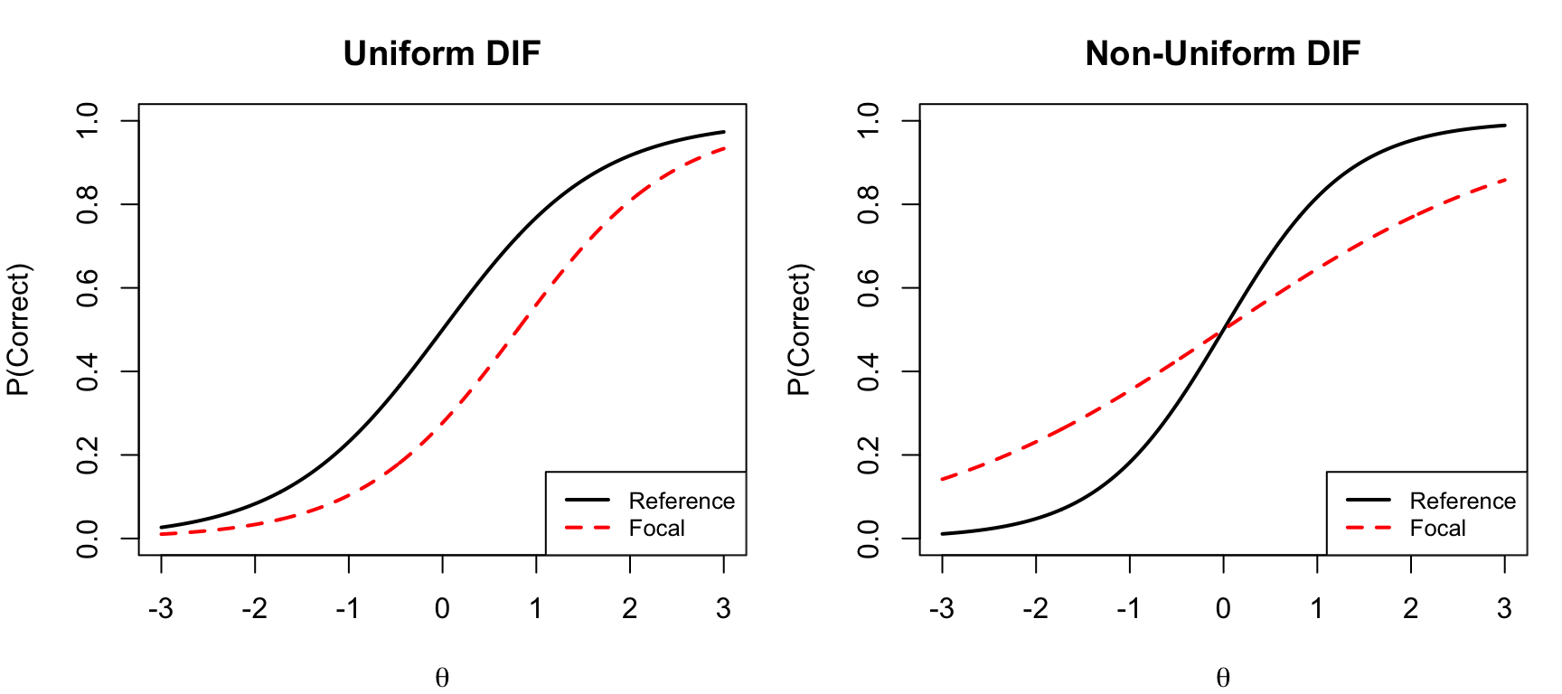
## Uniform vs. Non-Uniform DIF
DIF can be classified into two types based on how the item characteristic curves (ICCs) for two groups differ:
- **Uniform DIF**: One group is advantaged across the entire ability scale. In IRT terms, the ICCs for the two groups differ only in their difficulty (location) parameter. The curves are shifted but do not cross.
- **Non-uniform DIF**: The relative advantage switches direction at some point on the ability scale. In IRT terms, the ICCs differ in their discrimination (slope) parameter, and the curves cross. This is sometimes called "crossing DIF."
```{r dif-illustrations, fig.width=9, fig.height=4}
theta <- seq(-3, 3, 0.01)

par(mfrow = c(1, 2), mar = c(4, 4, 3, 1))

# Uniform DIF: different difficulty
p_ref <- 1 / (1 + exp(-1.2 * (theta - 0)))
p_foc <- 1 / (1 + exp(-1.2 * (theta - 0.8)))
plot(theta, p_ref, type = "l", lwd = 2,
     xlab = expression(theta), ylab = "P(Correct)",
     main = "Uniform DIF", ylim = c(0, 1))
lines(theta, p_foc, lwd = 2, lty = 2, col = "red")
legend("bottomright", c("Reference", "Focal"),
       lty = c(1, 2), col = c("black", "red"), lwd = 2, cex = 0.8)

# Non-uniform DIF: different discrimination
p_ref <- 1 / (1 + exp(-1.5 * (theta - 0)))
p_foc <- 1 / (1 + exp(-0.6 * (theta - 0)))
plot(theta, p_ref, type = "l", lwd = 2,
     xlab = expression(theta), ylab = "P(Correct)",
     main = "Non-Uniform DIF", ylim = c(0, 1))
lines(theta, p_foc, lwd = 2, lty = 2, col = "red")
legend("bottomright", c("Reference", "Focal"),
       lty = c(1, 2), col = c("black", "red"), lwd = 2, cex = 0.8)
par(mfrow = c(1, 1))
```
Non-uniform DIF is harder to detect and interpret because the direction of group advantage changes at different locations on the scale. Most DIF detection methods are primarily sensitive to uniform DIF.
## Evaluating DIF: A Two-Stage Process
Evaluating DIF involves two stages:
- **Stage 1**: Is there DIF? If yes, is the DIF both *statistically significant* and *practically significant*?
- **Stage 2**: What explains the DIF? This requires substantive judgment about item content, often involving expert review.
## Obstacles to Establishing DIF
Several practical obstacles complicate DIF detection:
- **Small sample sizes** limit statistical power to detect differences
- **Choice of matching criterion**: Should it be internal (total test score) or external? How do we know the matching criterion itself is unbiased?
- **The fundamental problem**: If ALL items on a test are biased against a focal group, no internal matching criterion can distinguish bias from impact. The utility of DIF analysis rests on the assumption that at least some items are unbiased.
- **DIF cancellation and amplification**: Individual items may show DIF in opposite directions, partially or fully canceling at the test level---or they may reinforce each other.
---
# Data
We will use data from the CDE mathematics test, a 31-item multiple-choice assessment. The data file also includes a gender indicator. The **focal group** is females and the **reference group** is males. The default when using `mantelhaen.test()` in R is for the lower alphanumeric value (females) to be designated the focal category and the higher value (males) the reference category.
```{r load-data}
fulldata <- read.fwf("CTBMathSci.rwo",
                     widths = c(rep(1, 76), 3, 1, 6), skip = 2)
cde <- fulldata[, c(1:31, 78)]
names(cde)[32] <- "gender"
```
Let's check the sample size by gender.
```{r gender-counts}
table(cde$gender)
```
There are `r sum(cde$gender == "F")` females and `r sum(cde$gender == "M")` males in the data.
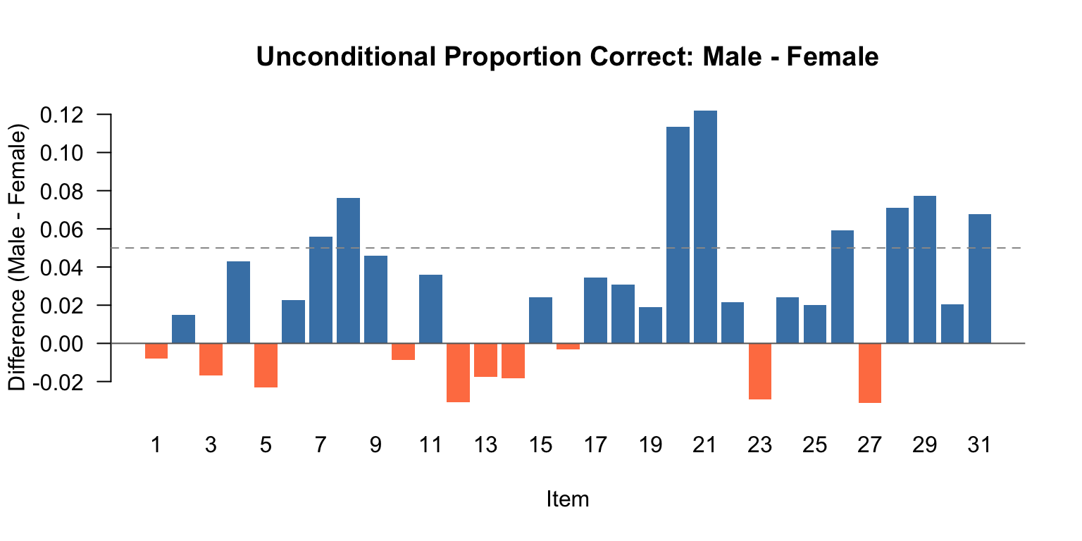
## Unconditional Item Performance by Gender
Before running any DIF analysis, it is good practice to examine the unconditional proportions correct by gender. Items where one group does substantially better than another are ones to keep an eye on. The question is: could part of this observed difference be caused by bias in how the item was written, rather than true ability differences?
```{r unconditional-crosstabs}
library(kableExtra)

# Compute proportion correct by gender for each item
p_correct <- data.frame(
  Item = 1:31,
  Female = sapply(1:31, function(i) mean(cde[cde$gender == "F", i], na.rm = TRUE)),
  Male = sapply(1:31, function(i) mean(cde[cde$gender == "M", i], na.rm = TRUE))
)
p_correct$Diff <- p_correct$Male - p_correct$Female

p_correct |>
  kable(digits = 3, col.names = c("Item", "P(Female)", "P(Male)", "Diff (M-F)")) |>
  kable_styling(full_width = FALSE) |>
  row_spec(which(abs(p_correct$Diff) > 0.05), bold = TRUE)
```
Items with differences greater than 5 percentage points (shown in bold) are candidates for closer inspection. But remember: these are *unconditional* differences. An item that appears to favor one group might not show DIF once we condition on ability.
```{r diff-barplot, fig.width=8, fig.height=4}
diff_vals <- p_correct$Diff
bar_cols <- ifelse(is.na(diff_vals), "gray",
                   ifelse(diff_vals > 0, "steelblue", "coral"))
barplot(diff_vals, names.arg = 1:31,
        xlab = "Item", ylab = "Difference (Male - Female)",
        main = "Unconditional Proportion Correct: Male - Female",
        col = bar_cols, border = NA, las = 1)
abline(h = 0, col = "gray40")
abline(h = c(-0.05, 0.05), lty = 2, col = "gray60")
```
---
# The Mantel-Haenszel Approach
## Basic Strategy
The **Mantel-Haenszel (MH)** procedure is the most widely used non-IRT method for detecting DIF. The basic strategy is:
- Examine 2 x 2 crosstabs of group (focal vs. reference) by item score (correct vs. incorrect)
- **Condition** on a matching criterion with a fixed number of levels (typically total test score, possibly collapsed into bins)
- Estimate the factor by which the odds of getting the item correct change for the focal group relative to the reference group, *after controlling for the matching criterion*
### Terminology
- **Focal group**: The group we are concerned about experiencing bias (in our example, females)
- **Reference group**: The group that might be advantaged by the way items are written (in our example, males)
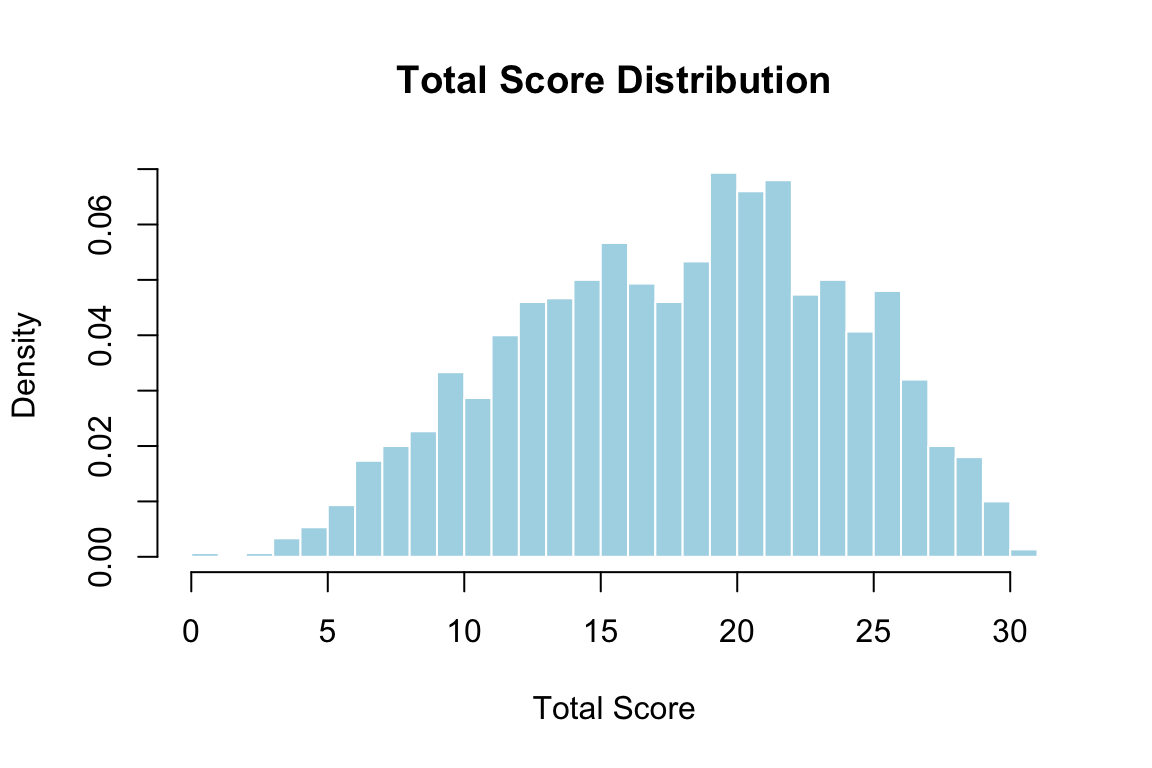
## Creating an Ability Grouping Variable
The MH procedure requires a discrete matching criterion. We use total test score, collapsed into bins to ensure adequate sample sizes at each level.
```{r mh-grouping}
totscore <- apply(cde[, 1:31], 1, sum)
```
Let's examine the total score distribution.
```{r totscore-dist, fig.width=6, fig.height=4}
hist(totscore, breaks = 0:31, freq = FALSE,
     main = "Total Score Distribution",
     xlab = "Total Score", col = "lightblue", border = "white")
```
We collapse scores into decile bins to keep sample sizes reasonably large at each level.
```{r create-bins}
x <- quantile(totscore, probs = seq(0, 1, 0.10))
diftot <- matrix(0, nrow(cde), 1)
for (i in 1:length(x) - 1) {
  diftot[(totscore >= x[i] & totscore < x[i + 1])] <- i
}
diftot[totscore == max(totscore)] <- length(x) - 1

table(diftot)
```
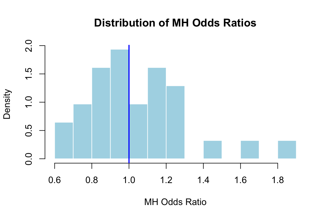
## Computing the MH Statistic
The MH statistic estimates a common odds ratio across all levels of the matching criterion. Under the null hypothesis, the odds of getting the item correct for the focal group are the same as for the reference group at every ability level. If the null is true, the odds ratio should equal 1.
- MH odds ratio **> 1**: The focal group (females) is *more* likely to answer correctly than comparable members of the reference group
- MH odds ratio **< 1**: The focal group is *less* likely to answer correctly than comparable members of the reference group
Let's compute the MH statistic for a single item first.
```{r mh-single}
mh <- mantelhaen.test(cde$V1, y = cde$gender, z = diftot,
                      alternative = "two.sided", conf.level = 0.95)
mh
```
Here the MH odds ratio is `r round(mh$estimate, 3)`. An odds ratio less than 1 means females are more likely to solve this item correctly than comparable males, but the result is not statistically significant.
Now we compute the MH statistic for all 31 items.
```{r mh-all}
MH <- list(NULL)
mh_or <- rep(0, 31)
mh_pval <- rep(0, 31)

for (i in 1:31) {
  temp <- mantelhaen.test(cde[, i], y = cde$gender, z = diftot,
                          alternative = "two.sided", conf.level = 0.95)
  MH[[i]] <- temp
  mh_or[i] <- temp$estimate
  mh_pval[i] <- temp$p.value
}
```
```{r mh-hist, fig.width=6, fig.height=4}
hist(mh_or, breaks = 15, freq = FALSE,
     main = "Distribution of MH Odds Ratios",
     xlab = "MH Odds Ratio", col = "lightblue", border = "white")
abline(v = 1, col = "blue", lwd = 2)
```
## The ETS Delta Statistic
The MH odds ratio is asymmetric around 1 (values favoring the reference group range from 0 to 1, while values favoring the focal group range from 1 to infinity). To produce a more interpretable, symmetric measure, Educational Testing Service (ETS) uses the **delta transformation**:
$$\Delta_{MH} = -2.35 \ln(\hat{\alpha}_{MH})$$
The delta statistic is interpreted as follows:
- **Negative values**: The reference group (males) found the item easier than the focal group (females) of comparable ability
- **Positive values**: The focal group (females) found the item easier than the reference group (males) of comparable ability
```{r ets-delta}
delta <- -2.35 * log(mh_or)
```
## ETS Classification Rules
ETS uses a three-level classification system for the practical significance of DIF:
- **Level A**: |delta| < 1 --- negligible DIF. Items are considered acceptable for use.
- **Level B**: 1 < |delta| < 1.5 --- moderate DIF. Items can be used with caution.
- **Level C**: |delta| > 1.5 --- large DIF. Items should not be used unless content experts can justify them.
```{r ets-classification}
level_A <- sum(abs(delta) <= 1)
level_B <- sum(abs(delta) > 1 & abs(delta) <= 1.5)
level_C <- sum(abs(delta) >= 1.5)

cat("Level A:", level_A, "items\n")
cat("Level B:", level_B, "items\n")
cat("Level C:", level_C, "items\n")
```
Let's create a summary table with the MH results and ETS classification for all items.
```{r mh-summary-table}
mh_results <- data.frame(
  Item = 1:31,
  OR = round(mh_or, 3),
  Delta = round(delta, 3),
  p_value = round(mh_pval, 4),
  Sig = ifelse(mh_pval < 0.05, "*", ""),
  Level = ifelse(abs(delta) >= 1.5, "C",
           ifelse(abs(delta) > 1, "B", "A"))
)

mh_results |>
  kable(col.names = c("Item", "MH OR", "Delta", "p-value", "Sig (.05)", "ETS Level")) |>
  kable_styling(full_width = FALSE) |>
  row_spec(which(mh_results$Level != "A"), bold = TRUE)
```
Notice that some items are statistically significant but not practically significant (Level A), and vice versa. The MH approach emphasizes both criteria for flagging items.
Also pay attention to the *direction* of DIF across flagged items. If all flagged items disadvantage the same group, the DIF may amplify at the test level. If the direction is mixed, DIF effects may partially cancel out.
## Limitations of the MH Approach
The MH procedure has several notable limitations:
- It uses total test score as the matching criterion, which may not be ideal if the Rasch model does not hold (i.e., items differ in discrimination)
- It requires collapsing the matching criterion into discrete bins, which may lose information
- It is primarily designed to detect **uniform DIF** and has limited power for **non-uniform DIF**
- It does not naturally incorporate an iterative purification process to account for DIF in the matching criterion itself
---
# Logistic Regression and DIF
Logistic regression provides a flexible bridge between the MH contingency table approach and IRT-based methods. As Swaminathan and Rogers (1990) showed, the MH procedure can be understood as a special case of logistic regression where the matching criterion is treated as a categorical variable. Moving to logistic regression gains us several advantages: the matching criterion can be treated as continuous, and we can explicitly test for both uniform and non-uniform DIF.
## Three Nested Models
For each item, we fit three nested logistic regression models:
- **Model 1**: $\text{logit}[P(Y = 1)] = \beta_0 + \beta_1 \cdot \text{ability}$
- **Model 2**: $\text{logit}[P(Y = 1)] = \beta_0 + \beta_1 \cdot \text{ability} + \beta_2 \cdot \text{group}$
- **Model 3**: $\text{logit}[P(Y = 1)] = \beta_0 + \beta_1 \cdot \text{ability} + \beta_2 \cdot \text{group} + \beta_3 \cdot \text{ability} \times \text{group}$
Comparing these models lets us test for:
- **Uniform DIF**: Compare Model 1 vs. Model 2 (1 df). A significant $\beta_2$ means the group variable shifts the intercept after controlling for ability.
- **Non-uniform DIF**: Compare Model 2 vs. Model 3 (1 df). A significant $\beta_3$ means the group-by-ability interaction changes the slope---the DIF effect varies across the ability scale.
- **Overall DIF**: Compare Model 1 vs. Model 3 (2 df). Tests for any type of DIF.
## Demonstration
Let's apply this to one item we flagged with MH (item 20) and one that appeared DIF-free (item 1).
```{r logistic-regression}
# Use continuous total score as matching criterion
totscore <- apply(cde[, 1:31], 1, sum)
gender <- cde$gender  # "F" = Female, "M" = Male

# --- Item 20 (flagged by MH) ---
m1_20 <- glm(cde$V20 ~ totscore, family = binomial)
m2_20 <- glm(cde$V20 ~ totscore + gender, family = binomial)
m3_20 <- glm(cde$V20 ~ totscore * gender, family = binomial)

cat("=== Item 20: Uniform DIF test (Model 1 vs 2) ===\n")
anova(m1_20, m2_20, test = "Chisq")
```
```{r logistic-item20-nonuniform}
cat("=== Item 20: Non-uniform DIF test (Model 2 vs 3) ===\n")
anova(m2_20, m3_20, test = "Chisq")
```
For item 20, we see a significant group effect (uniform DIF), consistent with the MH results.
```{r logistic-item1}
# --- Item 1 (not flagged by MH) ---
m1_01 <- glm(cde$V1 ~ totscore, family = binomial)
m2_01 <- glm(cde$V1 ~ totscore + gender, family = binomial)

cat("=== Item 1: Uniform DIF test (Model 1 vs 2) ===\n")
anova(m1_01, m2_01, test = "Chisq")
```
For item 1, there is no significant group effect, consistent with its Level A classification from the MH analysis.
## Connection to IRT-Based Approaches
The logistic regression framework is powerful because it can be extended in an important way: instead of using the observed total score as the matching criterion, we can substitute an **IRT-based trait estimate** ($\hat{\theta}$). This is exactly what the `lordif` algorithm does, and it has several advantages:
- IRT $\hat{\theta}$ accounts for differences in item discrimination, providing a better matching criterion
- IRT $\hat{\theta}$ is on a continuous, interval-like scale
- The iterative purification of $\hat{\theta}$ (re-estimating ability after accounting for DIF items) yields a cleaner matching criterion
---
# IRT-Based Approaches to DIF
## The Scale Indeterminacy Problem
Before we can compare ICCs across groups to look for DIF, we need to address a critical issue that connects directly to **test equating**---a topic we covered last week.
Suppose we calibrate a set of items separately for two groups and find that the ICCs look different. Can we conclude the items have DIF? **Not necessarily.** Recall that when we calibrate IRT models separately, the resulting scales are indeterminate---each group's parameters are on an arbitrary metric defined by the constraints imposed during estimation (typically, mean $\theta$ = 0, SD = 1 within each group).
If the two groups truly differ in their ability distributions (item impact), calibrating separately will absorb this difference into the item parameters, making it *look* like DIF when there is none.
### An Illustration
Imagine two groups take the same set of items. Group 1 has mean $\theta$ = 0, Group 2 has mean $\theta$ = 0.5. If we calibrate separately:
- Group 1 item parameters are estimated on a scale centered at 0
- Group 2 item parameters are estimated on a scale centered at 0
The true 0.5-unit difference in group means gets absorbed into the item difficulty estimates, making it appear that items are harder for Group 1---but this is just an artifact of scale indeterminacy.
### The Solution: Link the Scales First
Before comparing item parameters across groups, we must **link the two scales** using the same approaches covered in the test equating module:
- Identify a set of items believed to be **DIF-free** (analogous to anchor items in equating)
- Use these items to estimate linking constants (e.g., via the mean-sigma or Stocking-Lord method)
- Transform one group's parameters onto the other group's scale
- *Now* compare ICCs to look for genuine DIF
The challenge, of course, is that identifying DIF-free items requires first detecting DIF---which requires linked scales. This circular problem is addressed through **iterative purification**, which is precisely what the `lordif` algorithm implements.
---
## The lordif Algorithm
The `lordif` package (Choi, Gibbons, & Crane, 2011) implements an iterative hybrid approach that combines ordinal logistic regression with IRT. The algorithm proceeds through 11 steps:
1. **Data preparation**: Check for sparse cells in the cross-tabulation of items by group; collapse response categories as needed (controlled by `minCell` parameter).
2. **IRT calibration**: Fit the Graded Response Model (GRM) to the full dataset, ignoring group distinctions, to obtain a single set of item parameters. (The `lordif` package now uses `mirt` internally for this step.)
3. **Trait estimation**: Obtain $\hat{\theta}$ for each examinee using the Expected A Posteriori (EAP) estimator.
4. **Logistic regression**: For each item, fit the three nested logistic regression models (Models 1, 2, and 3) using the IRT-based $\hat{\theta}$ as the matching criterion. Compute likelihood ratio $\chi^2$ statistics, pseudo $R^2$ measures, and the proportional change in $\beta_1$.
5. **DIF detection**: Flag items based on the user-specified criterion (typically the $\chi^2$ test at $\alpha$ = 0.01).
6. **Sparse matrix construction**: For each flagged item, split the response vector into group-specific "pseudo-items" (e.g., responses for females with males set to missing, and vice versa). Non-DIF items remain intact.
7. **IRT recalibration**: Refit the GRM to the sparse data matrix, yielding common item parameters for non-DIF items and group-specific parameters for DIF items.
8. **Scale transformation**: Use the Stocking-Lord equating procedure (with non-DIF items as anchors) to place the group-specific parameters on a common scale.
9. **Trait re-estimation**: Obtain new EAP $\hat{\theta}$ estimates using the common parameters for non-DIF items and group-specific parameters for DIF items.
10. **Iterative cycle**: Repeat steps 4--9 until the same set of items is flagged on consecutive iterations or a maximum number of iterations is reached.
11. **Monte Carlo simulation** (optional): Generate datasets under the null hypothesis of no DIF (preserving observed group differences in $\hat{\theta}$) to obtain empirical distributions of the test statistics. This provides data-driven thresholds for flagging items rather than relying on fixed cutoffs.
---
## Running lordif on the CDE Data
```{r lordif-setup}
library(lordif)

response <- cde[, 1:31]
gender_num <- as.numeric(as.factor(cde$gender))
# as.factor converts "F"/"M" to factor levels; as.numeric makes Female = 1, Male = 2
```
Now we run the `lordif` algorithm using the likelihood ratio $\chi^2$ test as the detection criterion at $\alpha$ = 0.01.
```{r lordif-run, results='hide'}
dif_result <- lordif(response, gender_num,
                     criterion = "Chisqr", alpha = 0.01, minCell = 5)
```
### Examining the Results
```{r lordif-print}
print(dif_result)
```
The `print()` output shows which items were flagged for DIF, along with the $\chi^2$ statistics and pseudo $R^2$ values for each item. Let's examine the flagged items more carefully.
```{r lordif-flagged}
flagged_items <- dif_result$flag
cat("Items flagged for DIF:", which(flagged_items), "\n")
cat("Number of iterations:", dif_result$iteration, "\n")
```
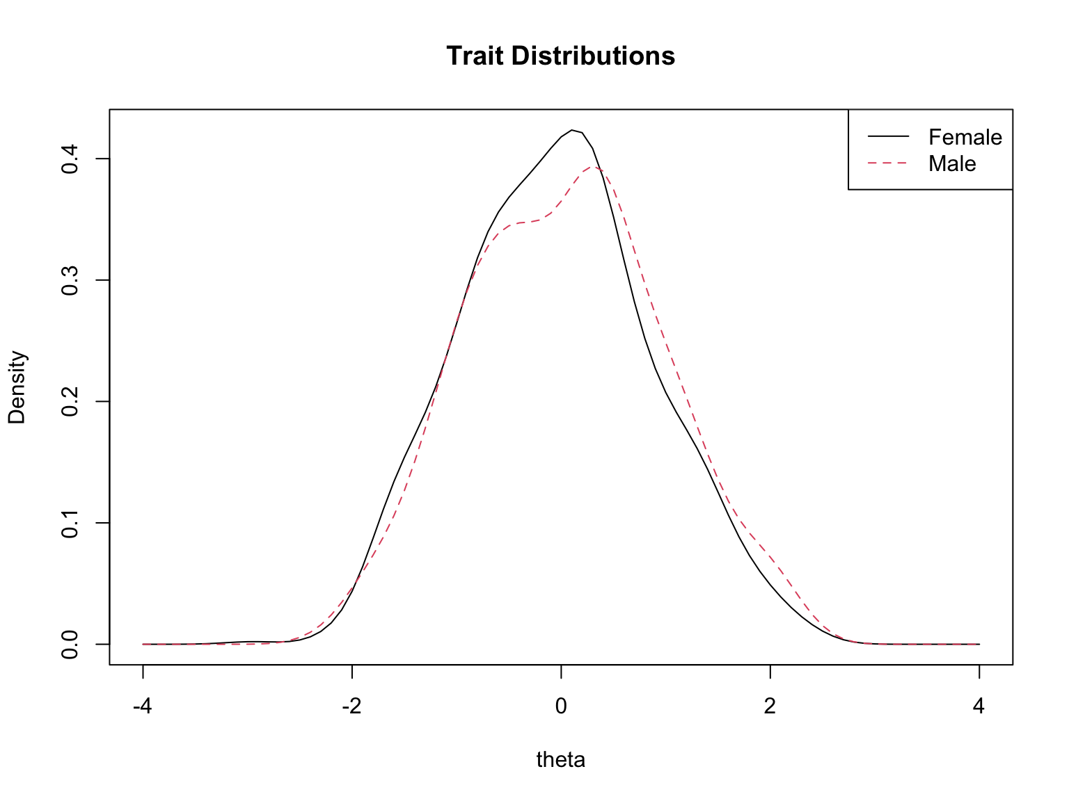
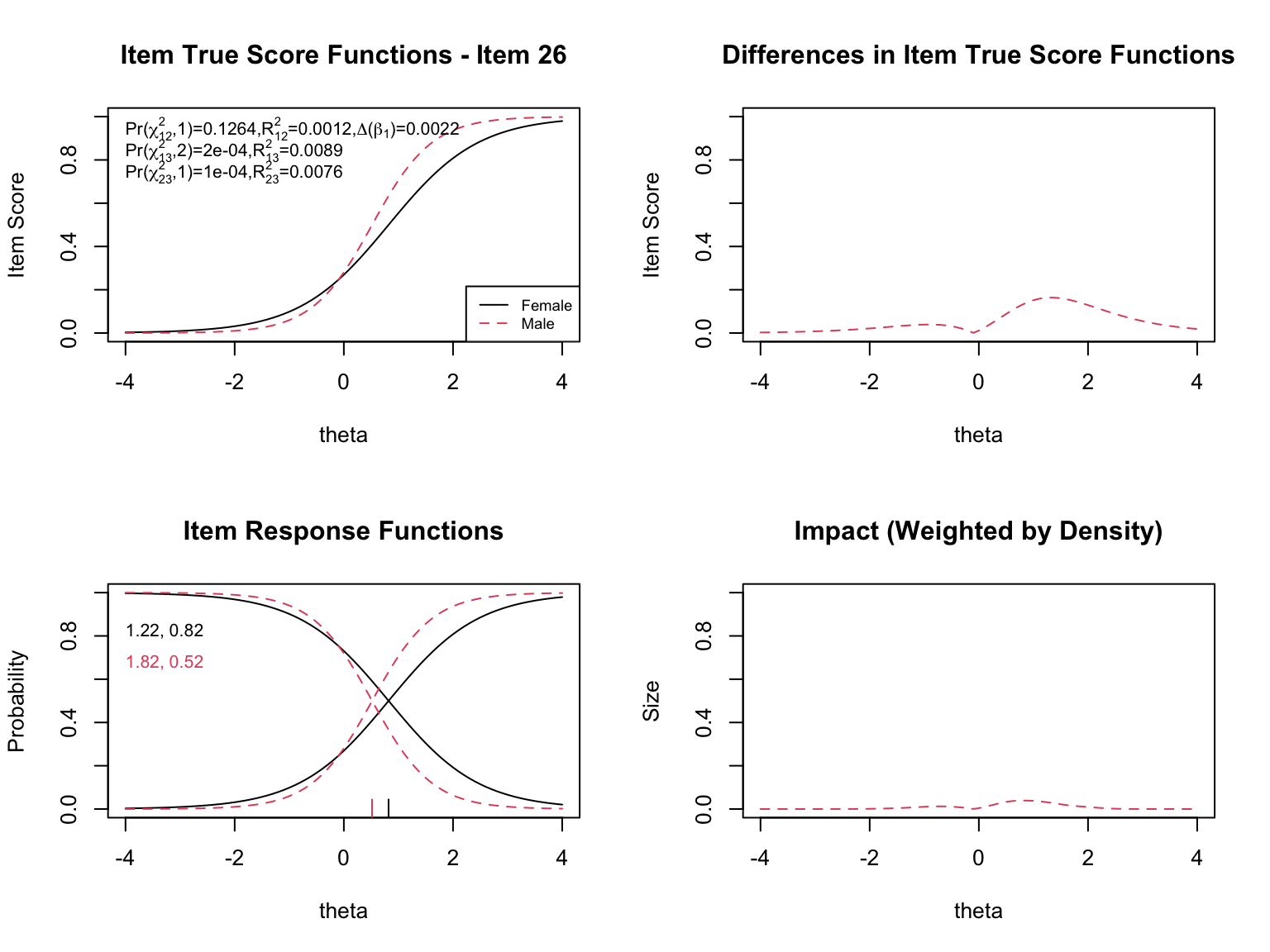
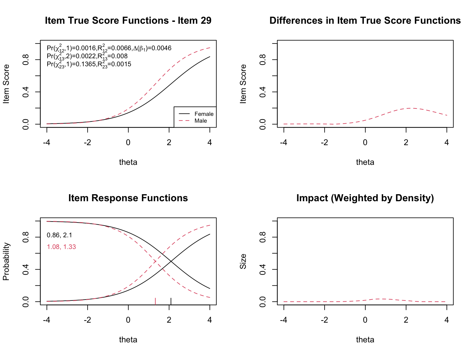
### Diagnostic Plots
The `plot()` function in `lordif` generates several types of diagnostic visualizations. First, it shows the trait distributions for the two groups (based on the final purified $\hat{\theta}$ estimates). Then, for each flagged item, it produces four diagnostic panels:
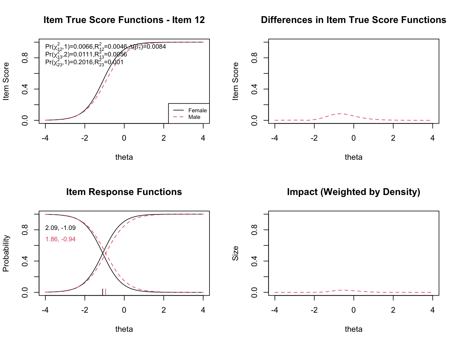
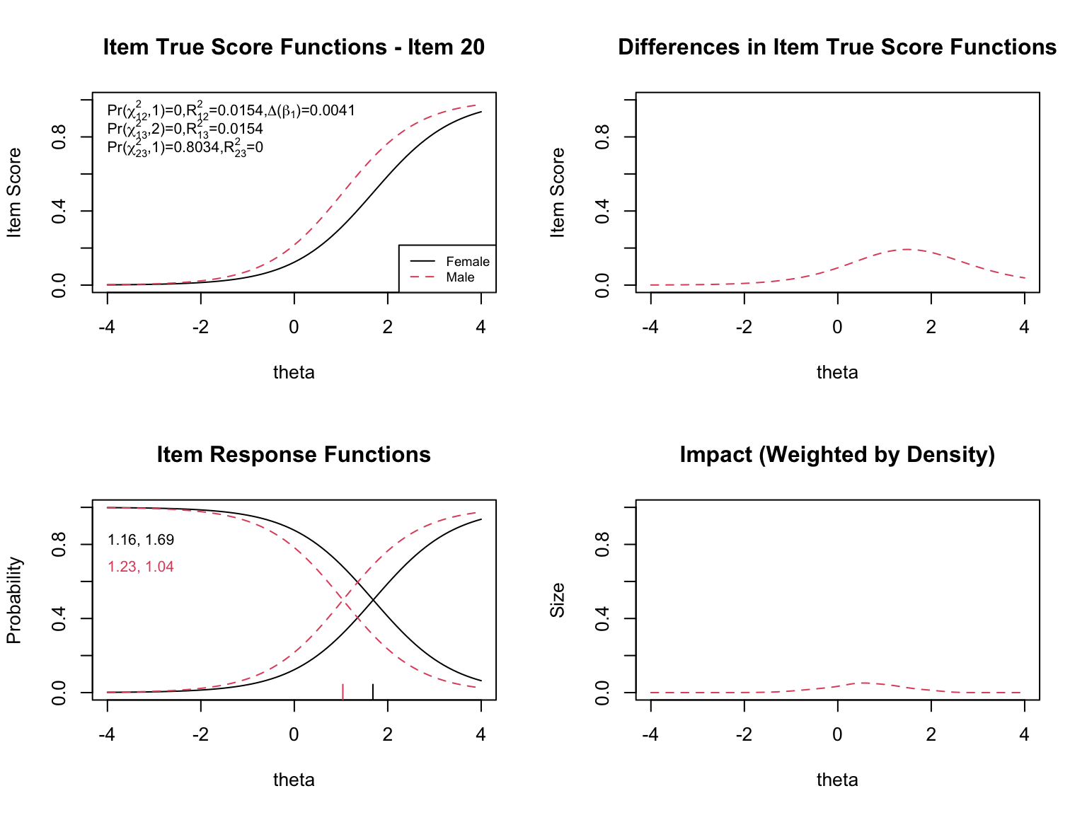
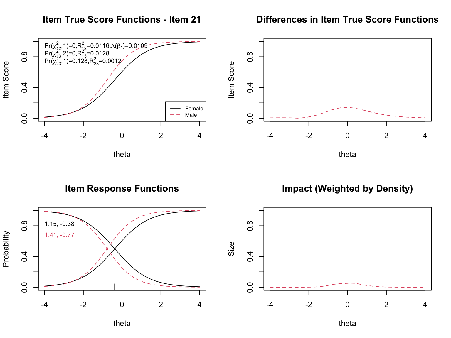
- **Top left**: Item true score functions by group (based on group-specific item parameters)
- **Top right**: Absolute difference between the group true score functions
- **Bottom left**: Item response functions by group (showing slope and threshold estimates)
- **Bottom right**: Impact weighted by the focal group density (showing where DIF matters most given the actual distribution of examinees)
```{r lordif-plots, fig.width=8, fig.height=6, results='hide'}
plot(dif_result, labels = c("Female", "Male"), cex = 0.7)
```
### Interpreting the Diagnostic Plots
When examining the plots for each flagged item, pay attention to:
- **Direction of DIF**: Which group is advantaged? Does the advantage hold across all ability levels (uniform) or does it reverse (non-uniform)?
- **Magnitude**: How large is the difference between the group-specific ICCs? Small differences may be statistically significant but practically negligible.
- **Impact**: The density-weighted plot (bottom right) shows where DIF actually matters given the population of examinees. An item might show a large ICC difference at extreme ability levels where few examinees exist, resulting in minimal practical impact.
- **The $\chi^2$ statistics**: The three tests (uniform, non-uniform, overall) printed on the top-left plot help classify the type of DIF.
- **The pseudo $R^2$ values**: These measure the magnitude of DIF. Values below 0.01 are generally considered negligible.
### Extracting Empirical Test- and Individual-Level Impact
In addition to the plots, we can pull a few numerical summaries directly from the `lordif` object to quantify the impact of DIF on the $\hat{\theta}$ estimates. Two components are particularly useful:
- `dif_result$calib$theta` --- the **initial** trait estimates, computed as if there were no DIF (common parameters for all items across groups).
- `dif_result$calib.sparse$theta` --- the **purified** trait estimates, computed with group-specific parameters for the flagged items.
Comparing these two sets of estimates tells us how much the individual (and group-mean) ability estimates change once DIF is accounted for.
```{r empirical-theta-shift}
theta_init <- dif_result$calib$theta          # ignoring DIF
theta_pur  <- dif_result$calib.sparse$theta    # accounting for DIF
se_pur     <- dif_result$calib.sparse$SE

m_init_F <- mean(theta_init[gender_num == 1])
m_init_M <- mean(theta_init[gender_num == 2])
m_pur_F  <- mean(theta_pur[gender_num == 1])
m_pur_M  <- mean(theta_pur[gender_num == 2])

cat("Initial theta  (no DIF adjustment):  F =", round(m_init_F, 3),
    " M =", round(m_init_M, 3),
    " M - F =", round(m_init_M - m_init_F, 3), "\n")
cat("Purified theta (DIF adjusted):       F =", round(m_pur_F, 3),
    " M =", round(m_pur_M, 3),
    " M - F =", round(m_pur_M - m_pur_F, 3), "\n")
# The initial single-group calibration anchors the theta metric to
# population mean 0 and SD 1, so these mean differences are already
# in population-SD units

shift <- theta_pur - theta_init
cat("Shift (purified - initial)\n")
cat("  Mean for F:", round(mean(shift[gender_num == 1]), 3),
    "  Mean for M:", round(mean(shift[gender_num == 2]), 3), "\n")
cat("  |shift| quantiles (50/75/95%):",
    round(quantile(abs(shift), c(0.5, 0.75, 0.95)), 3), "\n")
cat(" Max |shift|:", round(max(abs(shift)), 3), "logits\n")
cat(" Mean CSEM (purified theta):", round(mean(se_pur), 3), "logits\n")
```
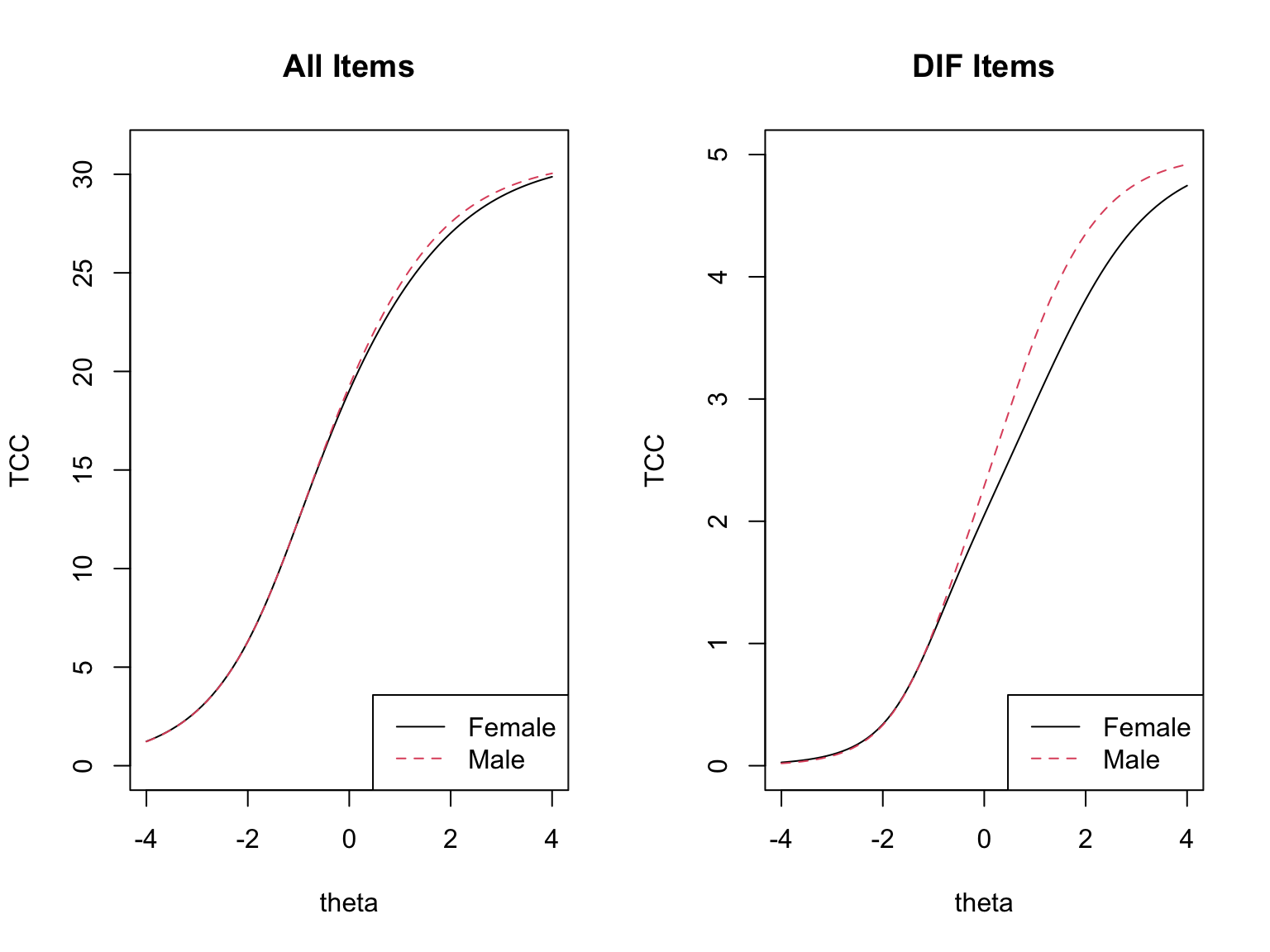
### Test-Level Impact
The test-level plots show the effect of DIF on the test characteristic curves (TCCs), and the group-mean comparison above quantifies the same thing numerically. The difference between the *initial* $\bar{\theta}_M - \bar{\theta}_F$ and the *purified* $\bar{\theta}_M - \bar{\theta}_F$ tells us how much of the apparent group gap was driven by DIF items rather than by true ability differences. To evaluate the **practical significance of DIF for aggregate group comparisons**, we express this difference in **population-SD units**. Because the initial single-group calibration identifies the latent metric with population mean 0 and SD 1, the raw mean $\hat{\theta}$ difference is already on this scale---no sample-based rescaling is needed (in fact, a sample-based denominator would be inappropriate, since EAP estimates shrink toward the prior and the pooled sample SD is systematically less than 1).
- If DIF operates in opposite directions across items, the effects **cancel** at the test level: the initial and purified group-mean differences are essentially the same and the TCCs are nearly coincident.
- If DIF is largely one-directional, the effects **amplify**: the purified difference is noticeably smaller (or larger) than the naive difference, and the TCCs clearly separate.
In the CDE data, the male advantage is about `r round(m_init_M - m_init_F, 2)` SD units under the naive calibration and about `r round(m_pur_M - m_pur_F, 2)` SD units after purification. A reduction of roughly `r round((m_init_M - m_init_F) - (m_pur_M - m_pur_F), 2)` SD units---approximately `r round(100 * ((m_init_M - m_init_F) - (m_pur_M - m_pur_F)) / (m_init_M - m_init_F))`% of the apparent gap---is attributable to DIF items rather than to true ability differences. This is partial amplification: not the full cancellation we see with balanced mixed-direction DIF, but not a wash either.
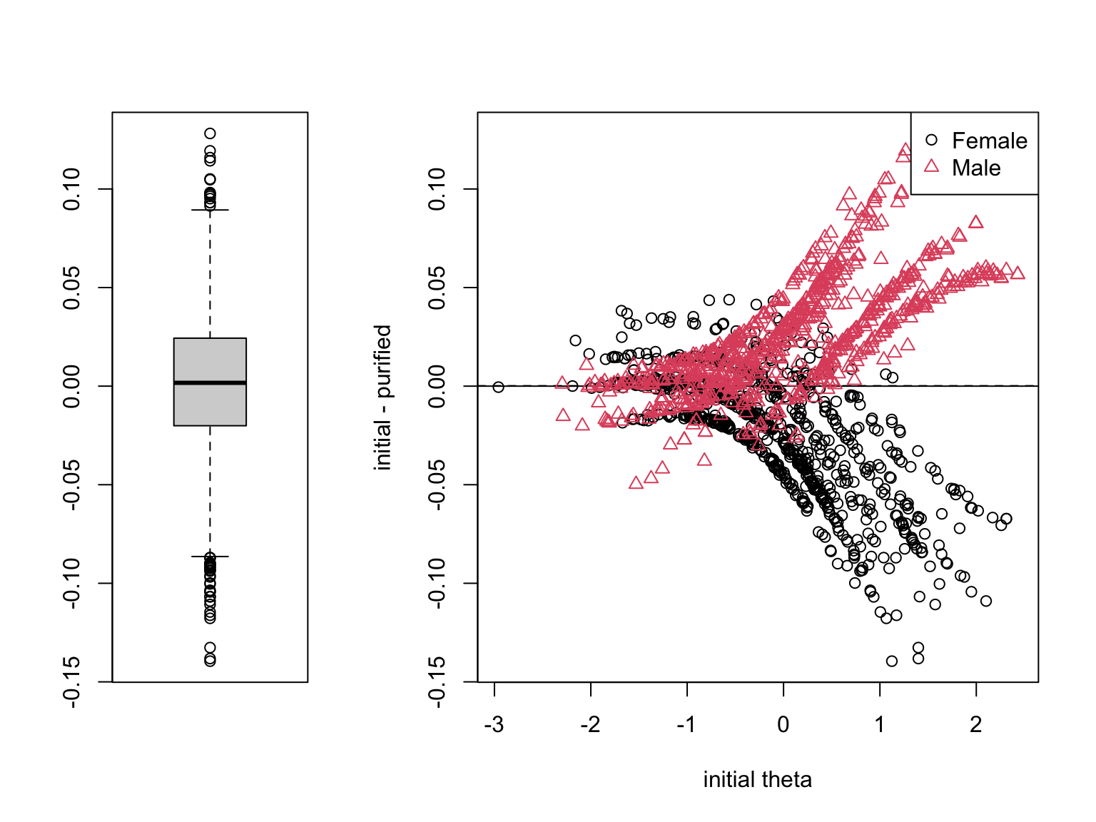
### Individual-Level Impact
The individual-level impact plot shows the initial $\hat{\theta}$ on the x-axis and the shift (purified $-$ initial) on the y-axis, in logits, with a boxplot summarizing the distribution. To judge the **practical significance of DIF for individual scores**, the relevant denominator is the **conditional standard error of measurement (CSEM)**. The CSEM already reflects the measurement uncertainty an individual estimate carries, so a DIF-induced shift much smaller than the CSEM is unlikely to change any single person's classification.
For the CDE data, the median absolute shift is about `r round(median(abs(shift)), 2)` logits, the 95th percentile is `r round(quantile(abs(shift), 0.95), 2)`, and the largest single shift is about `r round(max(abs(shift)), 2)` logits. The mean CSEM of the purified $\hat{\theta}$ is about `r round(mean(se_pur), 2)` logits. Typical shifts are a small fraction of a CSEM and therefore negligible at the individual level.
There is, however, an important caveat. Even when per-person shifts are tiny, their *direction* can be systematic by group. In the CDE data, the mean shift is about `r round(mean(shift[gender_num == 2]), 2)` logits for males and `r round(mean(shift[gender_num == 1]), 2)` logits for females---small, but pointing in opposite directions. Shifts that are uncorrelated across people would wash out in a group-mean comparison; **shifts that all point the same way within a group do not.** This is the mechanism through which small per-person shifts translate into the nontrivial group-level bias we saw above.
---
## Are the Differences Practically Significant?
Two benchmarks are relevant, and they answer different questions:
- **Population SD of $\theta$ (= 1 by the identification constraint of the initial calibration)** --- the right denominator for **group-level** comparisons. The change in the mean $\hat{\theta}$ difference from initial to purified estimates, read directly in SD units, expresses how much of the apparent group gap is DIF-induced. This is the benchmark that matters for the validity of inferences about group differences.
- **CSEM** --- the right denominator for **individual-level** interpretation. It reminds us that every individual estimate already carries substantial measurement error, so a shift well below the CSEM has little consequence for any one person's classification.
These two benchmarks can disagree in a way that is important to understand. When DIF cancels, both benchmarks give the same answer: effects are small. When DIF **amplifies**, the CSEM benchmark can make the effect look trivial (per-person shifts remain well below the SEM) while the population-SD benchmark correctly registers the systematic group-level bias. In other words, if individual $|$shifts$|$ are small but the group-mean difference changes appreciably from initial to purified, DIF is producing a **directional bias** at the group level---individuals move only a little, but they move in the *same* direction within each group, and those small shifts accumulate in group-mean comparisons. That is exactly the scenario in which a test can look measurement-invariant at the individual level while still misleading group-level inferences, and it is the validity concern that typically matters most.
---
# Comparing MH and lordif Results
```{r compare-methods}
mh_sig_items <- which(mh_pval < 0.05 & abs(delta) > 1)
lordif_items <- which(dif_result$flag)

cat("MH flagged items (sig + Level B/C):", sort(mh_sig_items), "\n")
cat("lordif flagged items: ", sort(lordif_items), "\n")
```
The two methods may not flag exactly the same items, for several reasons:
- **Different matching criteria**: MH uses observed total score; `lordif` uses IRT-based $\hat{\theta}$
- **Iterative purification**: `lordif` iteratively removes the influence of DIF items from the matching criterion; MH does not
- **Sensitivity to DIF type**: MH is primarily designed for uniform DIF; `lordif` can detect both uniform and non-uniform DIF
- **Scale linking**: `lordif` addresses scale indeterminacy through the equating step; MH does not
In general, items flagged by both methods are the strongest candidates for further review. Items flagged by only one method warrant closer examination to understand why.
---
# Summary
- **Impact**, **bias**, and **DIF** are distinct concepts. DIF is a necessary but not sufficient condition for item bias.
- The **Mantel-Haenszel** procedure is a widely used, computationally simple method for detecting uniform DIF. It uses an observed score as the matching criterion and produces the ETS delta statistic for practical significance classification.
- **Logistic regression** provides a flexible framework that can test for both uniform and non-uniform DIF by comparing nested models. It bridges the gap between contingency table methods and IRT-based approaches.
- **lordif** is an IRT-based method that uses ordinal logistic regression with IRT trait scores as the matching criterion. Its iterative purification process and scale transformation steps address key limitations of simpler methods.
- DIF detection depends on both **statistical** and **practical** significance. Items should be flagged only when both criteria are met.
- Almost all DIF methods use an **internal matching criterion**, which assumes that at least some items are unbiased.
- Finding DIF does not automatically mean an item is biased---**substantive expert review** is essential to determine whether the DIF reflects a genuine construct-irrelevant factor.
---
# References
- Choi, S., Gibbons, L., & Crane, P. (2011). lordif: An R Package for Detecting Differential Item Functioning Using Iterative Hybrid Ordinal Logistic Regression/Item Response Theory and Monte Carlo Simulations. *Journal of Statistical Software*, 39(8).
- Clauser, B. & Mazor, K. (1998). Using statistical procedures to identify differentially functioning test items. *Educational Measurement: Issues and Practice*, 17, 31--44.
- Holland, P. & Thayer, D. (1988). Differential item performance and the Mantel-Haenszel procedure. In H. Wainer & H. Braun (Eds.), *Test Validity* (pp. 129--145). Hillsdale, NJ.
- Swaminathan, H. & Rogers, H.J. (1990). Detecting differential item functioning using logistic regression procedures. *Journal of Educational Measurement*, 27, 361--370.
- Zwick, R. (2025). Fairness in Educational Measurement. In L. Cook & M. Pitoniak (Eds.), *Educational Measurement*, 5th Edition.