---
title: "Assumptions and Properties of IRT Models"
author: "Derek C. Briggs and Claude Code (Opus 4.6 & 4.7)"
output:
html_document:
toc: true
toc_float: true
code_folding: show
pdf_document:
toc: true
latex_engine: xelatex
---
```{r inject-rootdir, include=FALSE}
knitr::opts_knit$set(root.dir = "/Users/briggsd/Library/CloudStorage/Dropbox/Github/Measurement and Psychometrics/IRT Models for Dichotomously Scored Items/R Markdown Tutorials")
```
```{r setup, include=FALSE}
knitr::opts_chunk$set(echo = TRUE, message = FALSE, warning = FALSE)
# 3PL probability function (used throughout document)
calc_prob <- function(theta, a, b, c) {
c + (1 - c) * exp(a * (theta - b)) / (1 + exp(a * (theta - b)))
}
```
## Overview
IRT models rest on several key **assumptions** and have important **properties** that distinguish them from classical test theory. Understanding these is essential for proper application and interpretation.
| Assumptions | Properties |
|:------------|:-----------|
| Local Independence | Parameter Invariance |
| Appropriate Dimensionality | Scale Indeterminacy |
| Functional Form (ICC shape) | |
| Continuous latent variable | |
---
## Assumption 1: Local Independence
### Definition
Item responses are **statistically independent, conditional on the latent variable** $\theta$.
Put differently: the only reason item responses are correlated is due to their common dependence on $\theta$.
### Mathematical Expression
This assumption gives us the important result:
$$P(X_{1p} = 1 \text{ and } X_{2p} = 1 | \theta_p) = P(X_{1p} = 1 | \theta_p) \times P(X_{2p} = 1 | \theta_p)$$
More generally, for a full response pattern:
$$P(X_1, X_2, \ldots, X_I | \theta) = \prod_{i=1}^{I} P(X_i | \theta)$$
This is the same assumption made in factor analysis. For multidimensional IRT, we assume item responses are independent conditional on **all** dimensions of $\theta$ included in the model.
### Quick Aside: Useful Probability Rules
These rules are essential for understanding IRT:
1. **Complement Rule**: $P(A) = 1 - P(\neg A)$
- Probability of A is 1 minus the probability of A not happening
2. **Multiplication Rule (Independence)**: $P(A \text{ and } B) = P(A) \times P(B)$
- When A and B are independent
- This is the **joint probability** of A and B occurring
- Local independence allows us to use this for item responses
3. **Conditional Probability**: $P(A|B) = \frac{P(A \text{ and } B)}{P(B)}$
- Probability of A given that B happened
4. **Bayes' Rule**: $P(A|B) = \frac{P(B|A) \times P(A)}{P(B)}$
### What Causes Violations of Local Independence?
1. **Multidimensionality**: Test measures more than one latent trait
2. **Item chaining**: Answer to one item depends on previous item
3. **Testlet effects**: Items share common stimulus (e.g., reading passage)
4. **Speededness**: Time pressure creates dependence among later items
5. **Method effects**: Similar item formats create additional covariance
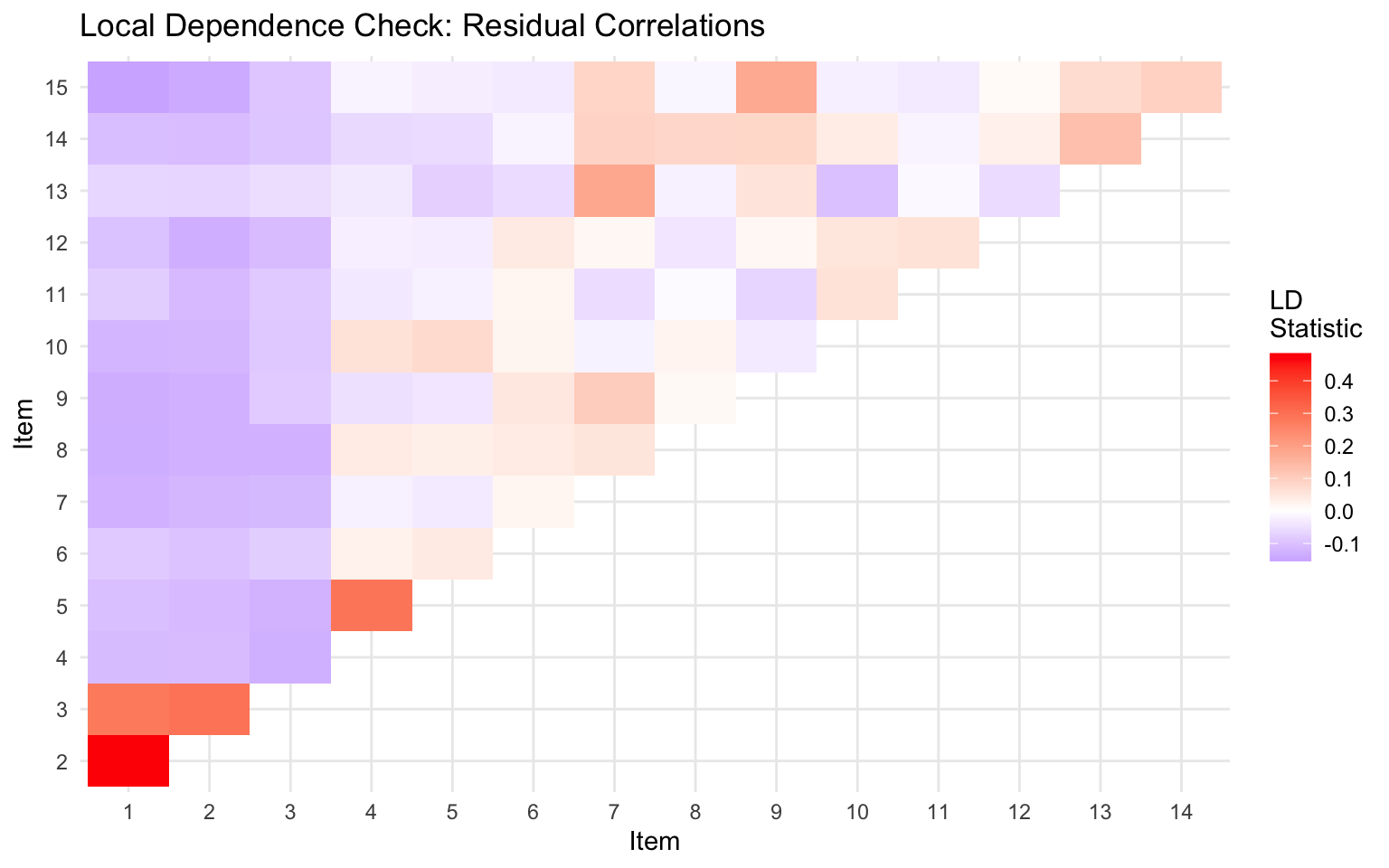
### Checking Local Independence
```{r check-li, fig.width=8, fig.height=5}
library(mirt)

# Load example data
forma <- read.csv("../Data/pset1_formA.csv")
forma <- forma[, 1:15]

# Fit model
mod <- mirt(forma, 1, itemtype = "2PL", verbose = FALSE)

# Residual correlations can indicate local dependence
# (suppress printed output - just keep the visualization)
residuals_ld <- suppressMessages(residuals(mod, type = "LD", verbose = FALSE))

# Visualize (upper triangle of matrix)
library(ggplot2)

# Convert to long format for plotting
ld_matrix <- as.matrix(residuals_ld)
ld_df <- expand.grid(Item1 = 1:15, Item2 = 1:15)
ld_df$LD <- as.vector(ld_matrix)
ld_df <- ld_df[ld_df$Item1 < ld_df$Item2, ]

ggplot(ld_df, aes(x = factor(Item1), y = factor(Item2), fill = LD)) +
  geom_tile() +
  scale_fill_gradient2(low = "blue", mid = "white", high = "red", midpoint = 0,
                       name = "LD\nStatistic") +
  labs(x = "Item", y = "Item", title = "Local Dependence Check: Residual Correlations") +
  theme_minimal()
```
Large positive values suggest items may be locally dependent.
---
## Assumption 2: Appropriate Dimensionality
### Definition
The model contains the **appropriate number of latent dimensions** to account for the covariance among items.
- For unidimensional IRT: One $\theta$ is sufficient
- For multidimensional IRT: Multiple $\theta$s are needed
### Key Points
- If a test is **multidimensional** and we fit only a single latent variable, this can cause **local item dependence**
- Dimensionality refers to the number of latent variables needed to model the response data
- This may or may not correspond to the hypothesized dimensionality of the theoretical construct
- Most IRT models used in practice are unidimensional
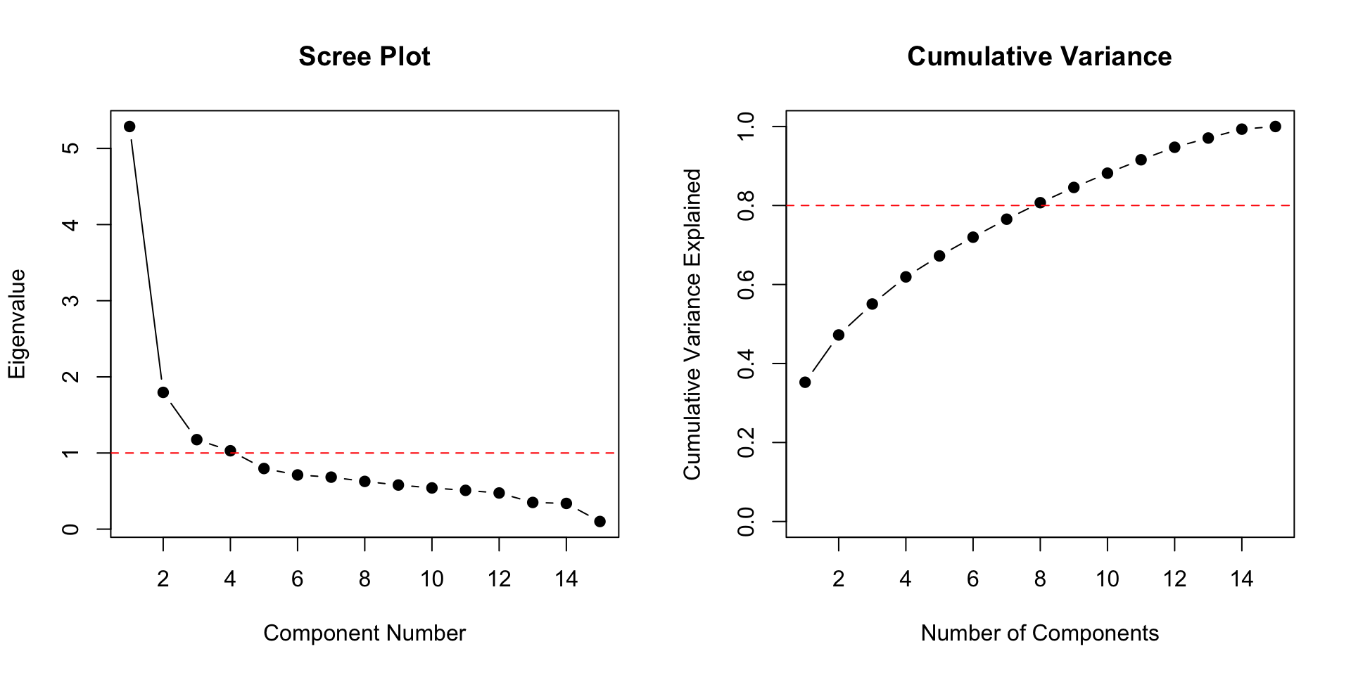
### Assessing Dimensionality
```{r dimensionality, fig.width=10, fig.height=5}
par(mfrow = c(1, 2))

# Eigenvalue plot (scree plot)
eigenvalues <- eigen(cor(forma))$values
plot(eigenvalues, type = "b", pch = 19,
     xlab = "Component Number", ylab = "Eigenvalue",
     main = "Scree Plot")
abline(h = 1, lty = 2, col = "red")

# Ratio of first to second eigenvalue
cat("First eigenvalue:", round(eigenvalues[1], 2), "\n")
cat("Second eigenvalue:", round(eigenvalues[2], 2), "\n")
cat("Ratio (1st/2nd):", round(eigenvalues[1]/eigenvalues[2], 2), "\n")
# Cumulative variance explained
cum_var <- cumsum(eigenvalues) / sum(eigenvalues)
plot(cum_var, type = "b", pch = 19,
     xlab = "Number of Components", ylab = "Cumulative Variance Explained",
     main = "Cumulative Variance", ylim = c(0, 1))
abline(h = 0.8, lty = 2, col = "red")
par(mfrow = c(1, 1))
```
**Guidelines:**
- A dominant first eigenvalue suggests unidimensionality
- Ratio of first to second eigenvalue > 3 often indicates essential unidimensionality
- But these are rough guidelines, not strict rules
---
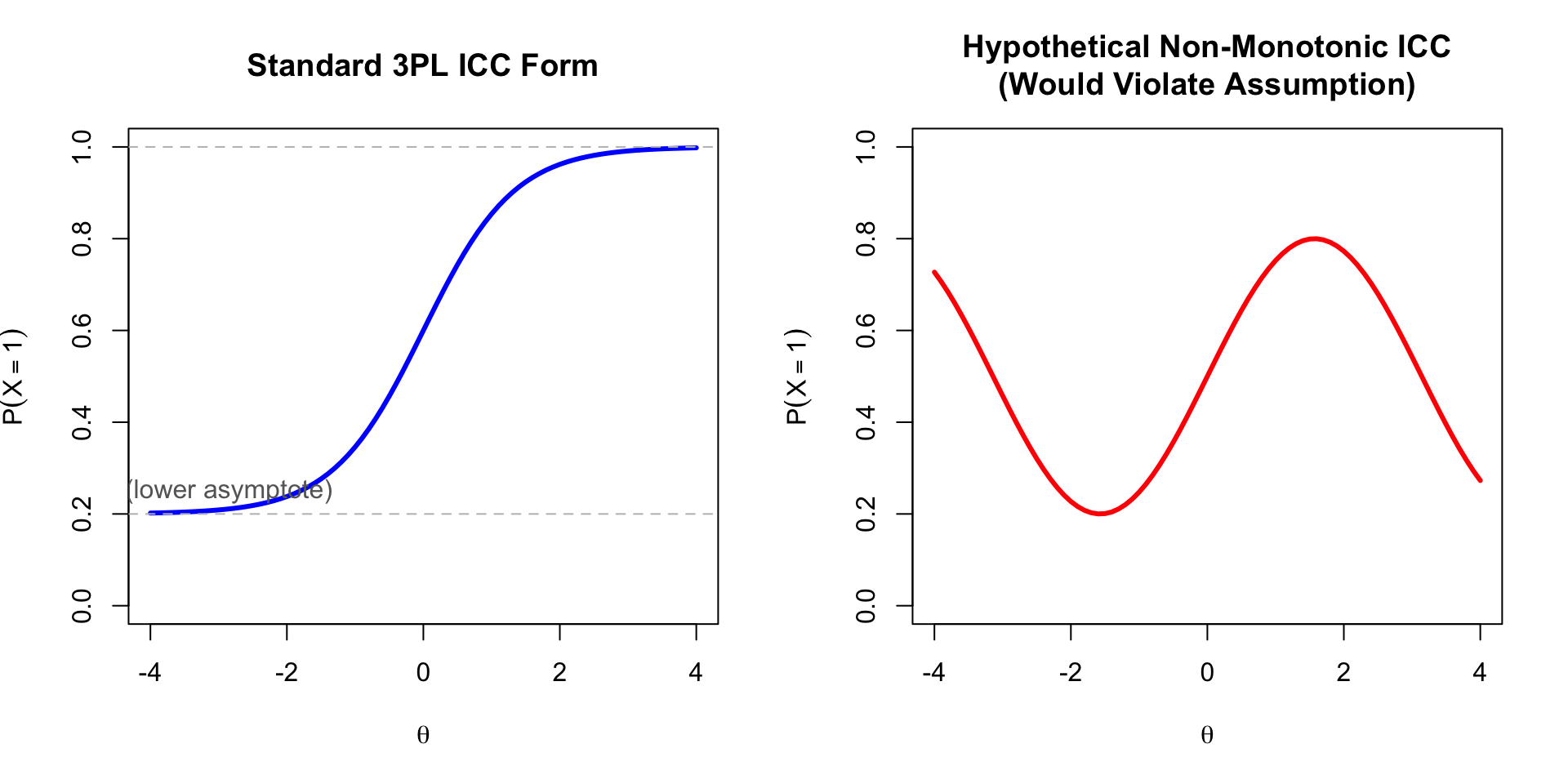
## Assumption 3: Functional Form (ICC Shape)
### Definition
We assume that the probability of correct responses follows the **logistic form** (or normal ogive):
$$P(X_{ip} = 1 | \theta_p) = c_i + (1 - c_i) \frac{\exp(a_i(\theta_p - b_i))}{1 + \exp(a_i(\theta_p - b_i))}$$
### Key Characteristics
1. **Monotonically increasing** probability as a function of $\theta$
2. **S-shaped** (sigmoidal) curve
3. Described by the $a$, $b$, and $c$ parameters
4. Lower asymptote determined by $c$
5. Upper asymptote is 1 (or can be less with a 4PL model)
```{r icc-form, fig.width=10, fig.height=5}
theta <- seq(-4, 4, 0.1)

par(mfrow = c(1, 2))

# Standard ICC
plot(theta, calc_prob(theta, 1.5, 0, 0.2), type = "l", lwd = 3, col = "blue",
     xlab = expression(theta), ylab = expression(P(X == 1)),
     main = "Standard 3PL ICC Form",
     ylim = c(0, 1))
abline(h = c(0.2, 1), lty = 2, col = "gray")
text(-3, 0.25, "c (lower asymptote)", col = "gray40")

# What if ICC were NOT monotonic? (This would violate the assumption)
theta_range <- seq(-4, 4, 0.1)
non_monotonic <- 0.5 + 0.3 * sin(theta_range)  # Hypothetical non-monotonic

plot(theta_range, non_monotonic, type = "l", lwd = 3, col = "red",
     xlab = expression(theta), ylab = expression(P(X == 1)),
     main = "Hypothetical Non-Monotonic ICC\n(Would Violate Assumption)",
     ylim = c(0, 1))
par(mfrow = c(1, 1))
```
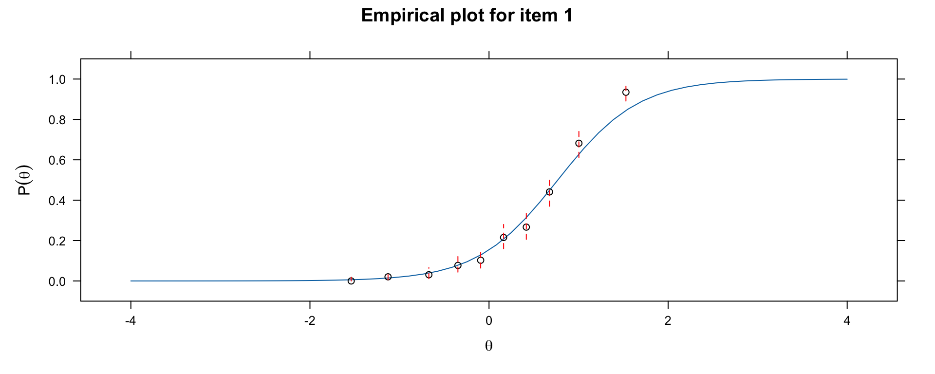
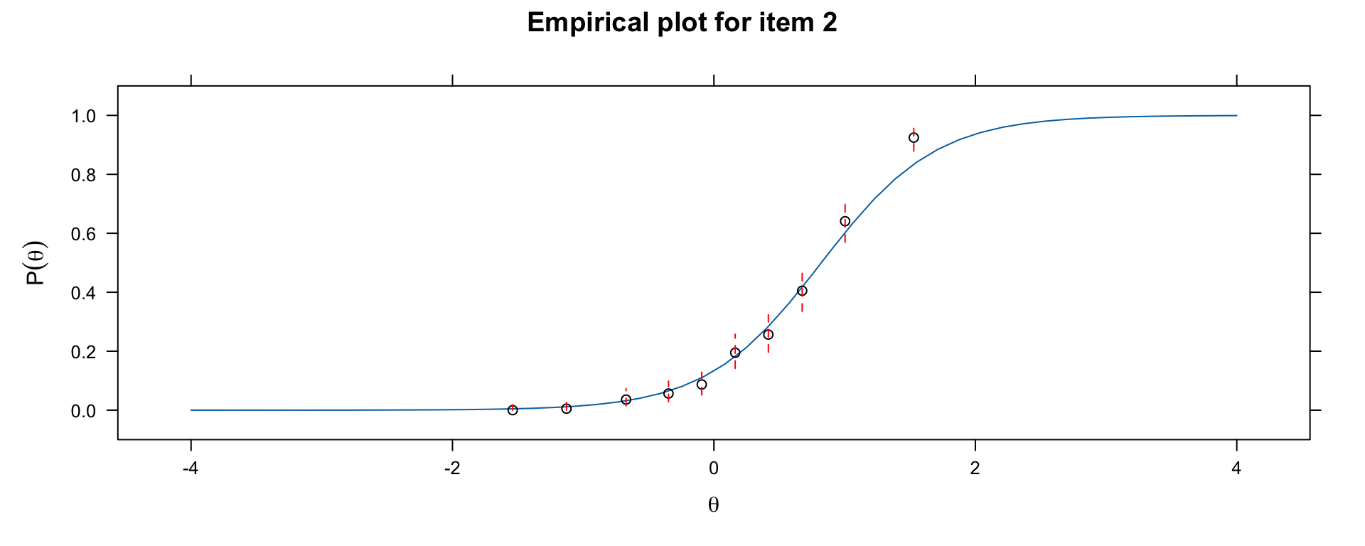
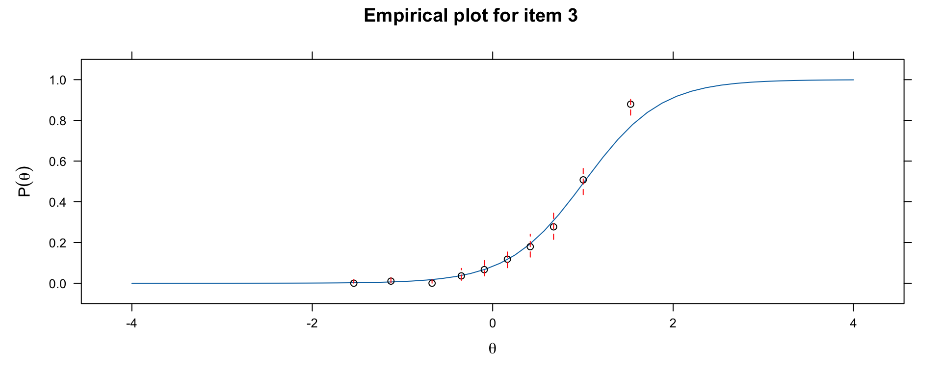
### Checking ICC Form with Empirical Plots
```{r empirical-icc, fig.width=10, fig.height=4}
# Compare model-implied ICC to empirical ICC
library(mirt)

par(mfrow = c(1, 3))

# Check item fit for 3 items
for (item in 1:3) {
  print(itemfit(mod, group.bins = 10, empirical.plot = item))
}
par(mfrow = c(1, 1))
```
If the empirical points deviate systematically from the model-implied curve, the functional form assumption may be violated.
---
## Property 1: Parameter Invariance
### Definition
If the model fits the data, **item parameter estimates should be the same regardless of the group used to estimate them**.
- We should get the same $a$, $b$, $c$ parameters whether we use high-ability or low-ability examinees
- Similarly, person parameters should be the same regardless of which items are used
### Why This Matters
| CTT | IRT |
|:----|:----|
| Item p-values depend on sample | Item parameters are invariant (if model fits) |
| Discrimination depends on sample variance | Discrimination is a stable property |
| Need matched samples for comparison | Can compare across different samples |
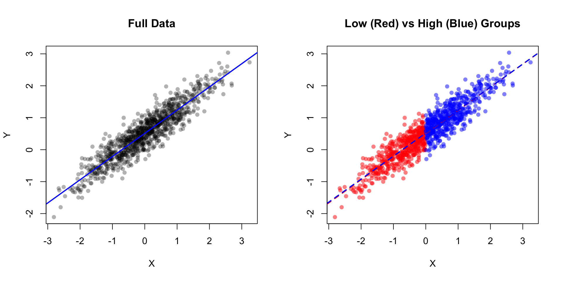
### Analogy: Linear Regression
In linear regression, we assume the slope and intercept are the same regardless of which subset of data we use to estimate them.
```{r invariance-demo, fig.width=10, fig.height=5}
set.seed(123)

# Generate population data
n <- 1000
x <- rnorm(n, 0, 1)
y <- 0.5 + 0.7 * x + rnorm(n, 0, 0.3)

# Split into "low" and "high" groups
low_group <- x < 0
high_group <- x >= 0

par(mfrow = c(1, 2))

# Full data
plot(x, y, pch = 16, col = rgb(0, 0, 0, 0.3),
     main = "Full Data", xlab = "X", ylab = "Y")
abline(lm(y ~ x), col = "blue", lwd = 2)

# Separate groups
plot(x[low_group], y[low_group], pch = 16, col = rgb(1, 0, 0, 0.5),
     xlim = range(x), ylim = range(y),
     main = "Low (Red) vs High (Blue) Groups", xlab = "X", ylab = "Y")
points(x[high_group], y[high_group], pch = 16, col = rgb(0, 0, 1, 0.5))
abline(lm(y[low_group] ~ x[low_group]), col = "red", lwd = 2, lty = 2)
abline(lm(y[high_group] ~ x[high_group]), col = "blue", lwd = 2, lty = 2)
par(mfrow = c(1, 1))

# Compare estimates
cat("Full data: slope =", round(coef(lm(y ~ x))[2], 3), "\n")
cat("Low group: slope =", round(coef(lm(y[low_group] ~ x[low_group]))[2], 3), "\n")
cat("High group: slope =", round(coef(lm(y[high_group] ~ x[high_group]))[2], 3), "\n")
```
---
## Property 2: Scale Indeterminacy
### The Problem
Because we cannot observe $a$, $b$, $c$, or $\theta$ directly, and they occur together in the model, there is **inherent indeterminacy** in the scale.
Consider the expression $a_i(\theta_p - b_i)$.
Now define new values:
- $b_i^* = (b_i + k_1) / k_2$
- $\theta_p^* = (\theta_p + k_1) / k_2$
- $a_i^* = k_2 \times a_i$
- $c_i^* = c_i$
It will be true that: $a_i(\theta_p - b_i) = a_i^*(\theta_p^* - b_i^*)$
### Resolving Scale Indeterminacy
There are two main approaches:
#### 1. Item-Side Anchoring
- Place constraints on item parameters (e.g., mean item difficulty = 0)
- Freely estimate the $\theta$ distribution
- More common in Rasch modeling and in Europe
#### 2. Person-Side Anchoring
- Fix distribution of $\theta$ to have mean = 0 and SD = 1
- Freely estimate item parameters
- More common in US and in achievement testing
### Practical Implications
1. **Comparing across studies**: Must ensure same scale/anchoring
2. **Linking**: Need anchor items or anchor persons to equate scales
3. **Interpretation**: The absolute value of $\theta$ is arbitrary; only relative positions matter
---
## Summary
### Assumptions
| Assumption | Description | Violation Consequences |
|:-----------|:------------|:-----------------------|
| Local Independence | Responses independent given $\theta$ | Biased parameter estimates |
| Dimensionality | Correct number of latent dimensions | Local dependence, poor fit |
| Functional Form | ICC follows logistic/normal ogive | Poor item fit |
| Continuous $\theta$ | Latent variable is continuous | (Rarely problematic) |
### Properties
| Property | Description | Practical Implication |
|:---------|:------------|:---------------------|
| Parameter Invariance | Parameters same across groups | Enables fair comparison |
| Scale Indeterminacy | Scale defined up to linear transform | Need anchoring conventions |
### Key Takeaways
1. **Local independence** is crucial - violations can seriously bias estimates
2. **Dimensionality** should be checked before fitting unidimensional models
3. **Parameter invariance** is a property, not an assumption - it holds if model fits
4. **Scale indeterminacy** means we need conventions to interpret parameters
5. Always check model assumptions before interpreting results!